How to Perform Grubbs’ Test in R

Grubbs’ Test, named after Frank E. Grubbs, is a statistical test used to detect outliers in a dataset. Outliers are those points in the dataset that differ from the rest of the dataset and do not follow a certain trend. These points can alter the analysis leading to incorrect solutions and predictions. Grubbs Test helps us to identify these outliers and give accurate results. In this article, we will understand how to perform Grubb’s Test in the R Programming Language.

What is Grubbs’ Test in R

Outliers can arise due to various reasons such as measurement errors, experimental errors, or genuine anomalies in the data. Dealing with them is necessary to provide accurate predictions otherwise due to these differing points our results might change. Grubb’s Test helps us to deal with these points ensuring the validity and reliability of statistical inferences. Grubbs’ Test provides a systematic approach to identifying outliers, enabling researchers and analysts to make informed decisions about their data. Below mentioned points will define the reason behind the use of Grubb’s Test:

1. Exploratory Data Analysis (EDA): This test is used to explore the dataset to understand the dataset in a better manner.
2. Quality Control: Grubb’s Test is used in fields such as manufacturing, healthcare, or environmental monitoring to identify potential issues.
3. Statistical Modeling: Outliers impact the statistical modeling therefore Grubbs’ Test is used to identify them.
4. Assumption Testing: Many statistical tests assume that the data is normally distributed. Grubbs’ Test helps in assessing this assumption by identifying outliers that may violate the normality assumption.

Mathematical Concept behind Grubb’s Test

Grubbs’ Test is based on the assumption that the dataset follows a normal distribution. The test statistic for Grubbs’ Test is calculated using the formula:

[Tex]G = \frac{\max_{i=1}^{n} |X_i – \mu|}{\sigma} [/Tex]

• G: This is the Grubbs’ test statistic.
• Xi​: Represents the individual data points in the dataset.
• μ: The mean (average) of the dataset. It is calculated by summing all the data points and dividing by the number of points.
• σ: The standard deviation of the dataset, measuring the dispersion or spread of the data points.
• maxi=1n​: This represents the maximum absolute deviation from the mean.

G represents the deviation of the suspected outlier from the mean in terms of standard deviations. The null hypothesis(H_o) taken in this case is that there is no outlier in the dataset. The above mentioned formula differs for the calculation of the max and min values.

What are Outliers and How to Deal with Them:

Outliers are the data points that deviate from the other points in dataset. These points can be extreme as well as some minor errors in the dataset but they affect the predictions. We can identify outliers with the help of graphs such as boxplot, scatter plots or histograms. These points that differ from the bulk points alter the statistical analyses and reduce the accuracy and precision of the prediction.

Dealing with Outliers

1. Omitting: Outliers can be removed from the dataset cautiously so that it does not affect the bulk points.
2. Transformation: We can transfer the dataset using mathematical concepts such as logarithmic transformation, this reduces the effect of these outliers
3. Robust Statistical Methods: robust regression or non-parametric tests can be used that are not much affected by the outliers as they are not sensitive to these data points.
4. Reporting: Transparency in dealing with these values is important. If outliers are identified in the dataset then we must deal, report their cause and discuss how they affect the entire dataset.

Grubbs’ Test on a car dataset:

Firstly, we will load and install ‘outliers’ package in R programming language to perform Grubb’s test

Load Required Libraries and Generate Sample Data:

Load and install the necessary packages and in this example, we are creating a fictional dataset by using set.seed()m function to create reproducibility in the dataset. We are taking three different models of cars along with their mpg(miles per gallon)

R

# Load required libraries library(outliers) # For Grubbs' Test library(ggplot2) # For data visualization # Generate fictional gas mileage data set.seed(123) # Setting seed for reproducibility car_models <- c(rep("SUV", 30), rep("Sedan", 30), rep("Hatchback", 30)) mpg <- c(rnorm(30, mean = 25, sd = 5), rnorm(30, mean = 30, sd = 4), rnorm(30, mean = 35, sd = 3)) # Generating gas mileage data gas_data <- data.frame(Model = car_models, MPG = mpg)

Visualize the Data

We will plot the dataset to identify and spot the outliers

R

# Visualize the Data: Boxplot to visualize gas mileage distribution by car model ggplot(gas_data, aes(x = Model, y = MPG, fill = Model)) + geom_boxplot() + # Adding boxplot layer labs(title = "Gas Mileage Distribution by Car Model", x = "Car Model", y = "Miles per Gallon") + # Adding labels and title theme_minimal() # Setting theme for the plot

Output:

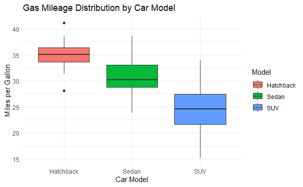
Grubbs’ Test in R

Perform Grubbs’ Test

Using Outliers package we will perform Grubbs’ Test on the given dataset

R

# Perform Grubbs’ Test grubbs_result <- grubbs.test(gas_data$MPG) # Print Grubbs' Test results print(grubbs_result)

Output:

Grubbs test for one outlier data: gas_data$MPG G = 2.66516, U = 0.91929, p-value = 0.2995 alternative hypothesis: lowest value 15.1669142168518 is an outlier

G: The test statistic (G) is 2.66516 indicating the deviation of the suspected outlier from the mean in terms of standard deviations.

• U: The critical value (U) is 0.91929, representing the maximum allowed deviation for the data not to be considered an outlier.
• p-value: The p-value is 0.2995, which is greater than the typical significance level of 0.05.

The output states that the lowest value (15.1669142168518) is identified as an outlier based on the test results. However, since the p-value is greater than 0.05, the significance of this outlier is not strong enough to reject the null hypothesis.

Identify Outliers

R

# Identify Outliers outliers <- gas_data$MPG[grubbs_result$outliers] # Extracting suspected outliers # Print suspected outliers print(outliers)

Output:

numeric(0)

No outliers were detected in the dataset based on the chosen significance level.

Grubbs’ Test on sales dataset

Here we are creating a fictional dataset based on the monthly sales of a retail chain for three years.

R

# Load required libraries library(outliers) # For Grubbs' Test library(ggplot2) # For data visualization # Step 1: Generate Synthetic Data set.seed(123) # Set seed for reproducibility months <- seq(as.Date("2022-01-01"), by = "month", length.out = 36) sales <- rnorm(36, mean = 50000, sd = 10000) # Generate normal sales data sales[c(5, 15, 25)] <- sales[c(5, 15, 25)] + c(30000, -20000, 40000) sales_data <- data.frame(Month = months, Sales = sales) # Create dataframe head(sales_data)

Output:

Month Sales 1 2022-01-01 44395.24 2 2022-02-01 47698.23 3 2022-03-01 65587.08 4 2022-04-01 50705.08 5 2022-05-01 81292.88 6 2022-06-01 67150.65

Visualize the Data

In this step with the help ggplot2 package in R programming language we are visualizing the dataset.

R

# Step 2: Visualize the Data ggplot(sales_data, aes(x = Month, y = Sales)) + geom_line(color = "blue") + geom_point(color = "red") + labs(title = "Monthly Sales Data", x = "Month", y = "Sales") + theme_minimal()

Output:

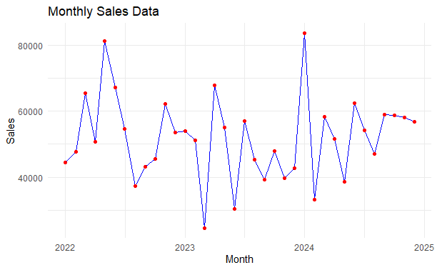
Grubbs’ Test in R

Identify Outliers

Best way to identify the outliers is to visualize them. In this step we are identify these outliers by a boxplot of monthly sales.

R

# Step 3: Identify Outliers Visually # Boxplot ggplot(sales_data, aes(x = NULL, y = Sales)) + geom_boxplot(fill = "lightblue", color = "black") + labs(title = "Boxplot of Monthly Sales", x = NULL, y = "Sales") + theme_minimal()

Output:

Grubbs’ Test in R

Perform Grubbs’ Test

Using outliers package and grubbs.test() function we are performing the test on the sales and the particular column we are concerned with.
print() function is used to display the result

R

# Step 4: Perform Grubbs' Test # Grubbs' Test grubbs_result <- grubbs.test(sales_data$Sales) # Print Grubbs' Test results print(grubbs_result)

Output:

Grubbs test for one outlier data: sales_data$Sales G = 2.50092, U = 0.81619, p-value = 0.1635 alternative hypothesis: highest value 83749.6073215074 is an outlier

Conclusion

In this article, we discussed the mathematical concept and the objective behind the calculation of Grubb’s Test and how we can deal the outliers with the help of multiple graphs and plots to identify these outliers.