Davies-Bouldin Index

Model evaluation is a crucial part of the machine learning process. When it comes to evaluating clustering in machine learning, optimizing the cluster count is a critical component. The Davies-Bouldin Index is a well-known metric to perform the same – it enables one to assess the clustering quality by comparing the average similarity between the pairwise most similar clusters. This article will explore the concepts related to the Davies-Bouldin Index and its implementation in Scikit-Learn.

Clustering

Clustering is a type of unsupervised machine learning that involves arranging/grouping the most similar data points into a fixed number of clusters. It is suitable for finding any structures or patterns within the data without requiring any prior knowledge about the grouping logic. It is very useful in segmentation tasks and finds a wide variety of applications like image compression, anomaly detection, and customer segmentation.

Davies-Bouldin Index

The Davies-Bouldin Index is a validation metric that is used to evaluate clustering models. It is calculated as the average similarity measure of each cluster with the cluster most similar to it. In this context, similarity is defined as the ratio between inter-cluster and intra-cluster distances. As such, this index ranks well-separated clusters with less dispersion as having a better score.

For a dataset , the Davies-Bouldin Index for k number of clusters can be calculated as

where:

is the intracluster distance within the cluster .

is the intercluster distance between the clusters .

The Davies-Bouldin index is very effective compared to other clustering evaluation metrics because:

• It is flexible and works for any number of clusters.
• It makes no assumptions about the shape of the clusters, unlike Silhouette Score evaluation metric.
• It is easy to use and intuitive.

Syntax

The davies_bouldin_score is provided within the sklearn.metrics module of the scikit-learn library. The following syntax is to be followed:

sklearn.metrics.davies_bouldin_score(X, labels)

• The method accepts two arguments – X (a list of data points with n features), and labels (a list of predicted labels for each of the n samples).
• The method returns a float value representing the Davies-Bouldin score for the given data.

How to calculate Davies-Bouldin Index?

1. Calculate the average distance between points in each cluster and the centroid of the cluster.
2. Calculate the distance between the centroids of each cluster and the nearest cluster.
3. Calculate the ratio of the average distance between points in a cluster and the centroid of the cluster to the distance between the centroids of the cluster and the nearest cluster.
4. Repeat steps 1-3 for each cluster.
5. Calculate the average of the ratios for all clusters.

Lower vs. Higher DB Index Values

The Davies-Bouldin Index (DBI) is a metric for evaluating the validity of a clustering solution. It is a relative clustering validity index, meaning that it compares the clustering results to a hypothetical “ideal” clustering. A lower DBI value indicates a better clustering solution.

• Higher DB index values correspond to poorer clustering solutions. This is because a higher DBI value indicates that the clusters are not well-separated and/or that the clusters are not compact.
• However, a lower DB index value is desirable. It indicates that the clusters are well-separated and compact, which is often a good indication of a successful clustering solution.

Implementation

Below is the Python implementation of DB index using the sklearn library

Scikit-Learn – Scikit-Learn is a popular Python3 library that provides a variety of methods to enable implementation of machine learning techniques like clustering, regression and classification. It provides various model evaluation scores, such as the Davies-Bouldin score, as part of its sklearn.metrics module.

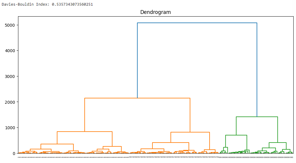
The code performs Agglomerative Hierarchical Clustering (AHC) on the Wine dataset and calculates the Davies-Bouldin Index (DBI) to evaluate the clustering results. It also plots a dendrogram to visualize the hierarchical structure of the data.

Python3

from sklearn.datasets import load_wine
from sklearn.cluster import AgglomerativeClustering
from sklearn.metrics import davies_bouldin_score
from scipy.cluster.hierarchy import dendrogram, linkage
import matplotlib.pyplot as plt

# Load the Wine dataset
wine = load_wine()
data = wine.data

# Perform Agglomerative Hierarchical Clustering
agg_clustering = AgglomerativeClustering(n_clusters=3)
agg_clustering.fit(data)

# Get the cluster labels
labels = agg_clustering.labels_

# Calculate Davies-Bouldin Index
db_index = davies_bouldin_score(data, labels)
print(f"Davies-Bouldin Index: {db_index}")

# Create a linkage matrix for dendrogram
linkage_matrix = linkage(data, method='ward')

# Plot the dendrogram
plt.figure(figsize=(12, 6))
dendrogram(linkage_matrix, orientation="top", labels=labels, distance_sort='descending')
plt.title('Dendrogram')
plt.show()

Output:

Implementation 2

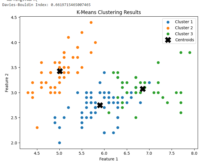
The code performs K-Means clustering on the Iris dataset and calculates the Davies-Bouldin Index (DBI) to evaluate the clustering results. It also plots a scatter plot to visualize the clustering results.

Python3

from sklearn.datasets import load_iris
from sklearn.cluster import KMeans
from sklearn.metrics import davies_bouldin_score
import matplotlib.pyplot as plt

# Load the Iris dataset
iris = load_iris()
data = iris.data

# Perform K-Means clustering
kmeans = KMeans(n_clusters=3)
kmeans.fit(data)

# Get the cluster labels
labels = kmeans.labels_

# Calculate Davies-Bouldin Index
db_index = davies_bouldin_score(data, labels)
print(f"Davies-Bouldin Index: {db_index}")

# Plot the clustering results in a scatter plot
plt.figure(figsize=(8, 6))

# Extract the centroids of each cluster
centroids = kmeans.cluster_centers_

# Scatter plot the data points with different colors for each cluster
for i in range(3):
    cluster_data = data[labels == i]
    plt.scatter(cluster_data[:, 0], cluster_data[:, 1], label=f'Cluster {i + 1}')

# Plot the centroids as well
plt.scatter(centroids[:, 0], centroids[:, 1], s=200, c='k', marker='X', label='Centroids')

plt.xlabel('Feature 1')
plt.ylabel('Feature 2')
plt.title('K-Means Clustering Results')
plt.legend()
plt.show()

Output:

Implementation 3

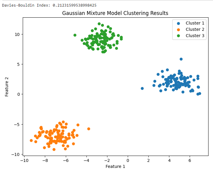
The code performs Gaussian Mixture Model (GMM) clustering on a synthetic dataset generated using scikit-learn’s make_blobs function. It also calculates the Davies-Bouldin Index (DBI) to evaluate the clustering results and plots a scatter plot to visualize the clustering results.

Python3

import numpy as np
from sklearn.datasets import make_blobs
from sklearn.mixture import GaussianMixture
from sklearn.metrics import davies_bouldin_score
import matplotlib.pyplot as plt

# Generate a synthetic dataset with blobs
n_samples = 300
n_features = 2
n_clusters = 3
random_state = 42

data, ground_truth_labels = make_blobs(n_samples=n_samples, n_features=n_features, centers=n_clusters, random_state=random_state)

# Perform Gaussian Mixture Model (GMM) clustering
gmm = GaussianMixture(n_components=n_clusters, random_state=random_state)
gmm.fit(data)

# Get the cluster labels
labels = gmm.predict(data)

# Calculate Davies-Bouldin Index
db_index = davies_bouldin_score(data, labels)
print(f"Davies-Bouldin Index: {db_index}")

# Plot the clustering results in a scatter plot
plt.figure(figsize=(8, 6))

# Scatter plot the data points with different colors for each cluster
for i in range(n_clusters):
    cluster_data = data[labels == i]
    plt.scatter(cluster_data[:, 0], cluster_data[:, 1], label=f'Cluster {i + 1}')

plt.xlabel('Feature 1')
plt.ylabel('Feature 2')
plt.title('Gaussian Mixture Model Clustering Results')
plt.legend()
plt.show()

Output:

Advantages of the Davies-Bouldin Index

1. The DBI is a relative metric, which means that it can be used to compare the clustering results of different algorithms on the same dataset.
2. The DBI has a clear interpretation: a lower DBI value indicates more compact and well-separated clusters.
3. It is a relatively simple metric to calculate.
4. It provides a global measure of the quality of a clustering solution.
5. It is relatively insensitive to the choice of distance metric.

Limitations of the Davies-Bouldin Index

1. The Davies-Bouldin Index is sensitive to outliers and noise in the data.
2. The Davies-Bouldin Index does not take into account the structure or distribution of data, such as clusters within clusters or non-linear relationships.
3. The Davies-Bouldin Index only considers the pairwise distances between cluster centroids and cluster members.
4. The DBI can be computationally expensive to calculate for large datasets.
5. The DBI is not suitable for all clustering tasks. For example, it is not well-suited for clustering tasks where the clusters are not well-separated.