In machine learning, decision trees are a popular tool for making predictions. However, a common problem encountered when using these models is overfitting. Here, we explore overfitting in decision trees and ways to handle this challenge.
Why Does Overfitting Occur in Decision Trees?
Overfitting in decision tree models occurs when the tree becomes too complex and captures noise or random fluctuations in the training data, rather than learning the underlying patterns that generalize well to unseen data. Other reasons for overfitting include:
- Complexity: Decision trees become overly complex, fitting training data perfectly but struggling to generalize to new data.
- Memorizing Noise: It can focus too much on specific data points or noise in the training data, hindering generalization.
- Overly Specific Rules: Might create rules that are too specific to the training data, leading to poor performance on new data.
- Feature Importance Bias: Certain features may be given too much importance by decision trees, even if they are irrelevant, contributing to overfitting.
- Sample Bias: If the training dataset is not representative, decision trees may overfit to the training data's idiosyncrasies, resulting in poor generalization.
- Lack of Early Stopping: Without proper stopping rules, decision trees may grow excessively, perfectly fitting the training data but failing to generalize well.
Strategies to Overcome Overfitting in Decision Tree Models
Pruning Techniques
Pruning involves removing parts of the decision tree that do not contribute significantly to its predictive power. This helps simplify the model and prevent it from memorizing noise in the training data. Pruning can be achieved through techniques such as cost-complexity pruning, which iteratively removes nodes with the least impact on performance.
Limiting Tree Depth
Setting a maximum depth for the decision tree restricts the number of levels or branches it can have. This prevents the tree from growing too complex and overfitting to the training data. By limiting the depth, the model becomes more generalized and less likely to capture noise or outliers.
Minimum Samples per Leaf Node
Specifying a minimum number of samples required to create a leaf node ensures that each leaf contains a sufficient amount of data to make meaningful predictions. This helps prevent the model from creating overly specific rules that only apply to a few instances in the training data, reducing overfitting.
Feature Selection and Engineering
Carefully selecting relevant features and excluding irrelevant ones is crucial for building a robust model. Feature selection involves choosing the most informative features that contribute to predictive power while discarding redundant or noisy ones. Feature engineering, on the other hand, involves transforming or combining features to create new meaningful variables that improve model performance.
Ensemble Methods
Ensemble methods such as Random Forests and Gradient Boosting combine multiple decision trees to reduce overfitting. In Random Forests, each tree is trained on a random subset of the data and features, and predictions are averaged across all trees to improve generalization. Gradient Boosting builds trees sequentially, with each tree correcting the errors of the previous ones, leading to a more accurate and robust model.
Cross-Validation
Cross-validation is a technique used to evaluate the performance of a model on multiple subsets of the data. By splitting the data into training and validation sets multiple times, training the model on different combinations of data, and evaluating its performance, cross-validation helps ensure that the model generalizes well to unseen data and is not overfitting.
Increasing Training Data
Providing more diverse and representative training data can help the model learn robust patterns and reduce overfitting. Increasing the size of the training dataset allows the model to capture a broader range of patterns and variations in the data, making it less likely to memorize noise or outliers present in smaller datasets.
Handling Overfitting in Decision Tree Models
In this section, we aim to employ pruning to reduce the size of decision tree to reduce overfitting in decision tree models.
Step 1: Import necessary libraries and generate synthetic data
Here , we generate synthetic data using scikit-learn's make_classification() function. It then splits the data into training and test sets using train_test_split().
import numpy as np
import matplotlib.pyplot as plt
from sklearn.datasets import make_classification
from sklearn.model_selection import train_test_split
from sklearn.tree import DecisionTreeClassifier
from sklearn.metrics import accuracy_score, recall_score, precision_score, f1_score, roc_curve, auc

# Generate synthetic data
X, y = make_classification(n_samples=1000, n_features=20, n_classes=2, random_state=42)

# Split data into training and test sets
X_train, X_test, y_train, y_test = train_test_split(X, y, test_size=0.2, random_state=42)
Step 2: Model Training and Initial Evaluation
This function trains a decision tree classifier with a specified maximum depth (or no maximum depth if None is provided) and evaluates it on both training and test sets. It returns the accuracy and recall scores for both sets along with the trained classifier.
def train_and_evaluate(max_depth=None):
    clf = DecisionTreeClassifier(max_depth=max_depth, random_state=42)
    clf.fit(X_train, y_train)
    y_pred_train = clf.predict(X_train)
    y_pred_test = clf.predict(X_test)

    train_accuracy = accuracy_score(y_train, y_pred_train)
    test_accuracy = accuracy_score(y_test, y_pred_test)

    train_recall = recall_score(y_train, y_pred_train)
    test_recall = recall_score(y_test, y_pred_test)

    return train_accuracy, test_accuracy, train_recall, test_recall, clf
Step 3: Visualization of Accuracy and Recall
Here the decision tree classifiers are trained with different maximum depths specified in the max_depths list. The train_and_evaluate() function is called for each maximum depth, and the accuracy and recall scores along with the trained classifiers are stored for further analysis.
plt.figure(figsize=(10, 5))

plt.subplot(1, 2, 1)
plt.plot(max_depths, train_accuracies, label='Training Accuracy')
plt.plot(max_depths, test_accuracies, label='Test Accuracy')
plt.xlabel('Maximum Depth')
plt.ylabel('Accuracy')
plt.title('Accuracy vs Maximum Depth')
plt.legend()

plt.subplot(1, 2, 2)
plt.plot(max_depths, train_recalls, label='Training Recall')
plt.plot(max_depths, test_recalls, label='Test Recall')
plt.xlabel('Maximum Depth')
plt.ylabel('Recall')
plt.title('Recall vs Maximum Depth')
plt.legend()

plt.tight_layout()
plt.savefig("accuracy_recall_plot.webp")
plt.show()
Output:
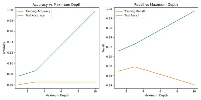
Accuracy Recall Plot
This plot shows how accuracy and recall vary with different maximum depths of decision tree classifiers. The plot is divided into two subplots: one for accuracy and the other for recall.
Step 5: Pruning Decision Trees
This part introduces cost-complexity pruning, an additional method to optimize decision trees by reducing their complexity after the initial training. It re-evaluates the pruned trees and visualizes their performance compared to the original unpruned trees.
pruned_train_accuracies = []
pruned_test_accuracies = []
pruned_train_recalls = []
pruned_test_recalls = []

pruned_classifiers = []

for clf in classifiers:
    path = clf.cost_complexity_pruning_path(X_train, y_train)
    ccp_alphas, impurities = path.ccp_alphas, path.impurities

    pruned_clfs = []

    for ccp_alpha in ccp_alphas:
        pruned_clf = DecisionTreeClassifier(random_state=42, ccp_alpha=ccp_alpha)
        pruned_clf.fit(X_train, y_train)
        pruned_clfs.append(pruned_clf)

    train_accuracies = [accuracy_score(y_train, clf.predict(X_train)) for clf in pruned_clfs]
    test_accuracies = [accuracy_score(y_test, clf.predict(X_test)) for clf in pruned_clfs]
    train_recalls = [recall_score(y_train, clf.predict(X_train)) for clf in pruned_clfs]
    test_recalls = [recall_score(y_test, clf.predict(X_test)) for clf in pruned_clfs]

    best_idx = np.argmax(test_accuracies)

    pruned_train_accuracies.append(train_accuracies[best_idx])
    pruned_test_accuracies.append(test_accuracies[best_idx])
    pruned_train_recalls.append(train_recalls[best_idx])
    pruned_test_recalls.append(test_recalls[best_idx])

    pruned_classifiers.append(pruned_clfs[best_idx])
Step 6: Comparing Accuracy and Recall before and after Pruning
plt.figure(figsize=(10, 5))

plt.subplot(1, 2, 1)
plt.plot(max_depths, train_accuracies[0:len(max_depths)], '--', label='Training Accuracy (Before Pruning)')
plt.plot(max_depths, test_accuracies[0:len(max_depths)], '--', label='Test Accuracy (Before Pruning)')
plt.plot(max_depths, pruned_train_accuracies, label='Training Accuracy (After Pruning)')
plt.plot(max_depths, pruned_test_accuracies, label='Test Accuracy (After Pruning)')
plt.xlabel('Maximum Depth')
plt.ylabel('Accuracy')
plt.title('Accuracy Before and After Pruning')
plt.legend()

plt.subplot(1, 2, 2)
plt.plot(max_depths, train_recalls[0:len(max_depths)], '--', label='Training Recall (Before Pruning)')
plt.plot(max_depths, test_recalls[0:len(max_depths)], '--', label='Test Recall (Before Pruning)')
plt.plot(max_depths, pruned_train_recalls, label='Training Recall (After Pruning)')
plt.plot(max_depths, pruned_test_recalls, label='Test Recall (After Pruning)')
plt.xlabel('Maximum Depth')
plt.ylabel('Recall')
plt.title('Recall Before and After Pruning')
plt.legend()

plt.tight_layout()
plt.savefig("accuracy_recall_before_after_pruning_plot.webp")
plt.show()
Output:
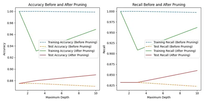
Accuracy Recall Before After Pruning Plot
It plot comparing accuracy and recall before and after pruning the decision tree classifiers. It shows two subplots: one for accuracy and the other for recall.
Step 7: Visualizing ROC curves for Pruned Classifiers
plt.figure(figsize=(8, 6))
for clf in pruned_classifiers:
    y_pred_prob = clf.predict_proba(X_test)[:, 1]
    fpr, tpr, thresholds = roc_curve(y_test, y_pred_prob)
    roc_auc = auc(fpr, tpr)
    plt.plot(fpr, tpr, label='AUC = %0.2f' % roc_auc)

plt.plot([0, 1], [0, 1], 'k--')  # random classifier curve
plt.xlim([0.0, 1.0])
plt.ylim([0.0, 1.05])
plt.xlabel('False Positive Rate')
plt.ylabel('True Positive Rate')
plt.title('Receiver Operating Characteristic (ROC) Curve')
plt.legend(loc="lower right")
plt.savefig("roc_curve_plot.webp")
plt.show()
Output:
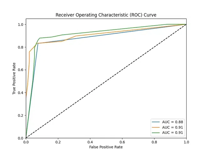
ROC Curve Plot
ROC curves for the pruned decision tree classifiers. The plot displays the true positive rate against the false positive rate, and the area under the curve (AUC) is calculated to evaluate the classifier's performance.
Conclusion
Decision trees are known for their simplicity in machine learning, yet overfitting causes a common challenge. This occurs when the model learns the training data too well but fails to generalize to new data. The code demonstrates how pruning techniques can address overfitting by simplifying decision trees. By comparing accuracy and recall before and after pruning, the effectiveness of these techniques is evident. Additionally, the recall curve visualization offers insight into the model's ability to distinguish between positive and negative cases.