What is Transfer Learning?
Transfer learning is a technique in deep learning where a pre-trained model on a large dataset is reused as a starting point for a new task. This approach significantly reduces training time and improves performance, especially when dealing with limited datasets.
It is very popular in computer vision and natural language processing as it makes it possible to leverage already trained models and then adjust them to match new tasks, usually on different amount of data and time.
Important Concepts of Transfer Learning
- Pre-trained models: These are deep learning models that have been pre-trained on the large datasets such as ImageNet for vision tasks, and these pre-trained models can be used by developers in transfer learning.
- Fine-tuning: With this technique, the pre-trained model will still be used as a basis for re-training with a new dataset that employs a very small learning rate just to be able to transfer it to a new task.
- Feature extraction: The second approach is referred to as the fine-tuning approach, which involves using the pre-trained model as a fixed feature extractor; here only the final classification layer is replaced during training.
- Normalize(mean=[0.5], std=[0.5]): Normalize the tensor by mean subtraction and standard devision. This is because it normalizes the input data by subtracting the mean and dividing it by the standard deviation which will be able to increase the speed of model training.
- Transformer: Transforms are a key data preprocessing stage in computer vision tasks, thus allow transforming the input data to the suitable form and scale so that the model can be processed efficiently. These Transform operations prove to be effective for the imaging of computer vision tasks, especially for deep learning models training and testing on image datasets.
Why Use Transfer Learning?
There are several compelling reasons to use transfer learning in machine learning, especially for deep learning tasks like image recognition or natural language processing:
- Reduced Training Time: Training complex deep learning models from scratch requires massive amounts of data and computational power. Transfer learning leverages a pre-trained model, significantly reducing the training time needed for a new task. Improved Performance (Especially with Limited Data): Deep learning models often suffer when trained on small datasets. Transfer learning mitigates this by incorporating knowledge from a large dataset, leading to better performance on the new task even with a limited amount of data specific to that task.
- Reduced Computational Resources: Training deep learning models necessitates significant computational resources. Transfer learning allows you to leverage a pre-trained model, reducing the computational burden required to train a model for your specific task. This is particularly beneficial when working with limited hardware resources.
- Faster Experimentation: By using transfer learning as a starting point, you can rapidly experiment with different model architectures and fine-tune them for your specific needs.
Pytorch for Transfer Learning
With PyTorch, the developers have an open source machine learning library for Python therein we experience the computational graph-based and dynamic approach that is flexible for building and training Neural Networks. It has the following features:
- Dynamic Computational Graph: While having an adaptable tensor flow visualization by design, Python Tire allows for the automatic formulation of tasks when operations are done. A static graph framework thus provides more robustness and faster debugging compared with the static ones.
- Tensor Computation: With the libraries of PyTorch, we have a powerful tool for the tensor calculus of the level of NumPy libraries, where a special feature is that it is done on GPU processing.
- Automatic Differentiation: PyTorch is equipped with some handy features- such as automatic differentiation property that makes it possible to calculate and handle gradients even with customized operations over the tensors. This is key for creation of the algorithm which will be gradient decent-based.
- Neural Network Building Blocks: PyTorch has a comprehensive range of functionalities to help with the development of neural networks such as pre-trained layers, activation functions, loss functions, and optimization levels.
- Dynamic Neural Networks: For example, PyTorch enables the trainable network of neurons to change structure as it runs, which makes complicated networks simple, like recurrent neural networks.
Usually, the PyTorch implementation is noted to be simple, adaptable, and wide-spread in the field of deep learning research and development for preferential prototyping and repeated experimentation.
Steps to Implement Transfer Learning for Image Classification in PyTorch
Transfer learning for image classification is essentially reusing a pre-trained neural network to improve the result on a different dataset. Follow the steps to implement Transfer Learning for Image Classification.
- Choose a pre-trained model (ResNet, VGG, etc.) based on your task.
- Modify the model by potentially replacing the final classification layer to match the number of classes in your new dataset.
- Freeze the pre-trained layers (make their weights non-trainable) to prevent them from being updated during training on the new dataset. This is especially useful when you have a small dataset.
- Preprocess your data, including resizing images and normalization.
- Optionally, perform data augmentation to increase the size and diversity of your dataset.
- Define the new model architecture by adding the new classifier on top of the pre-trained model.
- Compile the model by specifying the loss function, optimizer, and metrics.
- Train the model on your new dataset. Freezing the pre-trained layers might require fewer training epochs compared to training from scratch.
- Fine-tuning: You can further train the model by unfreezing some or all of the pre-trained layers.
- Evaluate the model's performance on a validation or test dataset to assess its accuracy and generalization capabilities.
Transfer Learning in PyTorch : Implementation
ResNet 50 Implementation
Here we are using Residual Networks (ResNet) demonstrating transfer learning for image classification on the MNIST dataset with a pre-trained ResNet-50 model.
Step 1: Choose a Pre-Trained Model
#Import neccessary libraries

import torch
from torchsummary import summary
import torch.nn as nn
import torch.optim as optim
import matplotlib.pyplot as plt
import torchvision.transforms as transforms
from torchvision.transforms import ToTensor, Normalize
from torchvision.datasets import MNIST, CIFAR10
from torch.utils.data import DataLoader

# Step 1: Choose a Pre-Trained Model
import torchvision.models as models

# Load the pre-trained ResNet-50 model
model = models.resnet50(pretrained=True)
Step 2: Modify the Model
class ModifiedResNet(nn.Module):
    def __init__(self):
        super(ModifiedResNet, self).__init__()
        self.resnet = torch.hub.load('pytorch/vision', 'resnet50', pretrained=True)
        num_classes = 10  # MNIST has 10 classes
        self.resnet.fc = nn.Linear(pretrained_model.fc.in_features, num_classes)  # Change the final fully connected layer for 10 classes

    def forward(self, x):
        return self.resnet(x)

model = ModifiedResNet()
Step 3: Freeze Pre-Trained Layers
for param in model.parameters():
    param.requires_grad = False
Step 4: Data Preprocessing
from torchvision.transforms.functional import pad

transform_train = transforms.Compose([
    transforms.RandomRotation(10),
    transforms.Grayscale(num_output_channels=3),  # Convert to RGB format
    transforms.ToTensor(),
    transforms.Normalize(mean=[0.5], std=[0.5])  # Normalize as before
])

transform_test = transforms.Compose([
    transforms.Grayscale(num_output_channels=3),  # Convert to RGB format
    transforms.ToTensor(),
    transforms.Normalize(mean=[0.5], std=[0.5])
])
Here is the breakdown of transformer functions used above:
- RandomResizedCrop(224): Randomly crop the image to 224x224 while the aspect ratio is retained. Use our AI to write for you about the importance of wildlife conservation. It comes also in handy during training time for data augmentation.
- RandomHorizontalFlip(): Flip the image horizontally randomly with a 0.5 probability. Last but not the least, another data augmentation method to render the variety in the training data.
- RandomRotation(10): Perform the maximum rotation of an image in random by 10 degrees. However another data augmentation method to making training data different which in turn can increase the variability of data.
- ToTensor(): Use the image as a PyTorch tensor. In PyTorch, the inputs of neural networks are supposed to be tensors.
- Grayscale(num_output_channels=3): Converts the image to grayscale, i.e. formating it through black and white. Arguments `num_output_channels=3` prevent degradation of image quality even if the input image is black-and-white.
Step 5: Data Augmentation
train_dataset = MNIST(root='./data', train=True, download=True, transform=transform_train)
train_loader = DataLoader(train_dataset, batch_size=128, shuffle=True)
Step 6: Define the Model Architecture
The code underneath is the same that was used in the creation of a ResNet model for transfer learning,here's a breakdown:
- `super(CustomResNet, self).__init__()`: Particularly in this particular line, there is meticulous care taken where the constructor of the parent class (the parent class here is `nn.Module`) is invoked to iteritialize the `CustomResNet` class.
- `self.resnet = torch.hub.load('pytorch/vision', 'resnet50', pretrained=True)`: This implies that we incorporate the model through the `torch.hub.load('pytorch/vision:v0.1', 'resnet50')`. The `pretrained` argument depicts that the mode is initialized with the precondition that we must give the files loaded with the pre-trained weights.
- `self.features = nn.Sequential(*list(pretrained_model.children())[:(`(fn.seq( [nn.Sequential( io.layer.(nn.select(-1)))] ))`: Meanwhile, the layer incl. the last layer (partially except last densely connected layer of the ResNet) is sequentialized. It is achieved by developing the framework from all the kids (which are filters of pretrained_models) and using them as parameters for nn.Sequential category of objects.
- `self.classifier = nn.Linear(pretrained_model.fc.in_features, 10)`: As a result, it generates a new fully connected layer (`nn.Linear`) which is titled as `classifier` that has the inputs being equal to the number of features in output of the final fully connected layer (`pretrained_model.fc.in_features`) of the ResNet model and the outputs that are ten (assuming the model takes ten classes to classify).
In general, an architecture model is constructed in the design of ResNet transfer learning where the initial layer is pre-trained and having been transferred to the ResNet feature layer the new layer is added for doing the specific classification task at the end.
class CustomResNet(nn.Module):
    def __init__(self, pretrained_model):
        super(CustomResNet, self).__init__()
        self.resnet = torch.hub.load('pytorch/vision', 'resnet50', pretrained=True)
        self.features = nn.Sequential(*list(pretrained_model.children())[:-1])
        self.classifier = nn.Linear(pretrained_model.fc.in_features, 10)

    def forward(self, x):
        x = self.features(x)
        x = x.view(x.size(0), -1)
        x = self.classifier(x)
        return x

model = CustomResNet(pretrained_model)
Step 7: Compile the Model
criterion = nn.CrossEntropyLoss()
optimizer = optim.Adam(model.parameters(), lr=0.001)
summary(model,(3,32,32))
Step 8: Train the Model
# Enable gradient computation for the last few layers
for param in model.resnet.layer4.parameters():
    param.requires_grad = True

# Train the model
model.train()
Step 9: Fine-Tuning
# Fine-tuning
num_epochs = 10
train_losses = []
train_correct = 0
train_total = 0
for epoch in range(num_epochs):
    model.train()
    running_loss = 0.0
    for inputs, labels in train_loader:
        optimizer.zero_grad()
        outputs = model(inputs)
        loss = criterion(outputs, labels)
        loss.backward()
        optimizer.step()
        running_loss += loss.item()

        _, predicted = torch.max(outputs, 1)
        train_total += labels.size(0)
        train_correct += (predicted == labels).sum().item()

    train_losses.append(running_loss / len(train_loader.dataset))
    train_accuracy = train_correct / train_total
    print(f'Epoch {epoch + 1}/{num_epochs}, Loss: {running_loss / len(train_loader)}')

print(f'Finished fine-tuning with {train_accuracy} accuracy')
Output:
        Epoch 1/10, Loss: 0.11688484001491688
        Epoch 2/10, Loss: 0.048869684821109906
        Epoch 3/10, Loss: 0.03598501617416565
        Epoch 4/10, Loss: 0.02836105151862494
        Epoch 5/10, Loss: 0.02060385358987499
        Epoch 6/10, Loss: 0.018268288789577147
        Epoch 7/10, Loss: 0.015551028832140913
        Epoch 8/10, Loss: 0.0124812169526237
        Epoch 9/10, Loss: 0.011541623044260112
        Epoch 10/10, Loss: 0.010758856865840513
        Finished fine-tuning with 0.9904533333333333 accuracy
Step 10: Evaluate the Model
test_dataset = MNIST(root='./data', train=False, download=True, transform=transform_test)
test_loader = DataLoader(test_dataset, batch_size=128, shuffle=False)  # Don't shuffle test data

# Initialize variables for tracking performance
test_losses = []
correct = 0
total = 0

# Loop through epochs for testing
for epoch in range(num_epochs):
    with torch.no_grad():
        running_loss = 0.0

        # Evaluate the model on the test set
        for images, labels in test_loader:
            # Forward pass (no need for gradients during testing)
            outputs = model(images)

            # Calculate loss (assuming your loss function is defined)
            loss = criterion(outputs, labels)

            # Update running loss
            running_loss += loss.item()

            # Calculate accuracy
            _, predicted = torch.max(outputs.data, 1)  # Get the index of the maximum value
            total += labels.size(0)
            correct += (predicted == labels).sum().item()

        # Calculate average loss for the epoch
        test_loss = running_loss / len(test_loader.dataset)
        test_losses.append(test_loss)

    # Print epoch-wise performance (optional)
    print(f'Epoch {epoch+1} - Test Loss: {test_loss:.4f}')

# Calculate and print overall test accuracy
test_accuracy = correct / total
print(f'Accuracy of the model on the test set: {test_accuracy:.4f}')
Output
Epoch 1 - Test Loss: 0.0002
Epoch 2 - Test Loss: 0.0002
Epoch 3 - Test Loss: 0.0002
Epoch 4 - Test Loss: 0.0002
Epoch 5 - Test Loss: 0.0002
Epoch 6 - Test Loss: 0.0002
Epoch 7 - Test Loss: 0.0002
Epoch 8 - Test Loss: 0.0002
Epoch 9 - Test Loss: 0.0002
Epoch 10 - Test Loss: 0.0002
Accuracy of the model on the test set: 0.9933
Step 11: Model Deployment
We deploy Transfer Learning by the following
- First we preprocess QMNIST images to convert them to tensors and normalize them.
- Then we take samples from QMNIS test dataset and DataLoader to evaluate model performances.
- We deploy the trained model with the data of QMNIST in order to check whether they work properly.
- Being the model accuracy checker, it compares the labels of the model with its predictions.
- Output the detail of the accuracy for the model on QMNIST dataset.
# Define the transformation for QMNIST
transform_qmnist = transforms.Compose([
    transforms.Resize(224),
    transforms.Grayscale(num_output_channels=3),  # Convert to 3 channels
    transforms.ToTensor(),
    transforms.Normalize((0.1307,), (0.3081,))
])


# Download and create a DataLoader for the QMNIST test set
qmnist_test_dataset = QMNIST(root='./data', what='test', download=True, transform=transform_qmnist)
qmnist_test_loader = DataLoader(qmnist_test_dataset, batch_size=128, shuffle=False)
qmnist_test_labels = qmnist_test_dataset.targets

# Deploy the model on the QMNIST dataset
predictions_qmnist = []
with torch.no_grad():
    for images, _ in qmnist_test_loader:
        outputs = model(images)
        _, predicted = torch.max(outputs, 1)
        predictions_qmnist.extend(predicted.tolist())

# Display or use the results
print("Predictions for QMNIST test set:", predictions_qmnist)

correct_qmnist = sum(p == gt for p, gt in zip(predictions_qmnist, qmnist_test_labels))
total_qmnist = len(predictions_qmnist)
accuracy_qmnist = correct_qmnist / total_qmnist
Output:
Predictions for CIFAR-10 test set: [9, 1, 1, 7, 5, 0, ...... 1, 5, 6, 5, 5]VGG16 Implementation
Similarly, we can also Implement VGG16 model, by replacing the architecture for implementing Tranfer Learning on CIFAR-10 Dataset.
Here is the implementation below:
Step 1: Choose a Pre-Trained Model
#Import neccessary libraries

import torch
from torchsummary import summary
import torch.nn as nn
import torch.optim as optim
import matplotlib.pyplot as plt
import torchvision.transforms as transforms
from torchvision.transforms import ToTensor, Normalize
from torchvision.datasets import MNIST, CIFAR10, CIFAR100
from torch.utils.data import DataLoader

# Step 1: Choose a Pre-Trained Model
import torchvision.models as models

# Load the pre-trained VGG16 model
model = models.vgg16(pretrained=True)
Step 2: Modify the Model
# Load and modify the model
num_classes= 10                     #Class size of MNIST dataset
model = models.vgg16(pretrained=True)
num_features = model.classifier[6].in_features
model.classifier[6] = nn.Linear(num_features, num_classes)
Step 3: Freeze Pre-Trained Layers
for param in model.parameters():
    param.requires_grad = False
Step 4: Data Preprocessing
# Data Preprocessing
transform_train = transforms.Compose([
    transforms.Resize((224, 224)),  # Resize images to (224, 224) for VGG-16
    transforms.ToTensor(),
    transforms.RandomCrop(32, padding=4),
    transforms.RandomHorizontalFlip(),
    transforms.ToTensor(),
    transforms.Normalize((0.5, 0.5, 0.5), (0.5, 0.5, 0.5)),
])

transform_test = transforms.Compose([
    transforms.Resize((224, 224)),  # Resize images to (224, 224) for VGG-16
    transforms.ToTensor(),
    transforms.Normalize((0.5, 0.5, 0.5), (0.5, 0.5, 0.5)),
])
Step 5: Data Augmentation
train_dataset = MNIST(root='./data', train=True, download=True, transform=transform_train)
train_loader = DataLoader(train_dataset, batch_size=128, shuffle=True)

test_dataset = MNIST(root='./data', train=False, download=True, transform=transform_test)
test_loader = DataLoader(test_dataset, batch_size=128, shuffle=False)  # Don't shuffle test data
Step 6: Define the Model Architecture
Here is the code overview of VGG16 Architecture:
1. `class VGG16(nn.Module):`
- It is equivalent to say `VGG16 as a new class which inherits from nn.Module,` it says it is a neural network that builds on top of the PyTorch framework.
2. `def __init__(self):`
- Make the method called `VGG16()` within `make_model()` function, which is used for instance generation.
- `super(VGG16, self).__init__()`: Uses the respective `__init__` methods of the `Module` and `nn.Module` classes to ensure the creation of the model model.
3. `self.features = vgg16(pretrained=True).features`
- Then, loads the VGG16 model with `vgg16` model weight pre-train( `pretrained =True`), then only takes the feature extraction part ( `features`) of the model.
- `self.features` is defined to matches `VGG16`'s pre-trained model feature extractor's features.
4. `self.avgpool = nn.AdaptiveAveragePool2d((7,7))`
- Among others, I would select the `nn.AdaptiveAvgPool2d`, which is often used in the processing of images. This section is where the adaptive average pooling layer takes the stage and does its best. Another way that convolutional layers scale down these maps and of the size is the fixed size of the 7x7 features.
- Adaptive pooling layer is generally prior to the classifier so that the classifier may have an independent input size of generated image.
5. `self.classifier = nn.Sequential(...)`
- In the following function a layer of classifier and labeling component is generated with nn.Sequential which is an object and it can put several layers in succession easily.
- These `nn.Linear` layers with `nn.ReLU` activation and `nn.Dropout` in between the classifier, are arranged in a non-linear manner.
- The number of neurons that each one sends to the next layer is set equal to `512*7*7`, corresponding to 7*7 pixels, indicating the lateral size of the second layer.
class MiniVGG(nn.Module):  # Smaller VGG for MNIST
  def __init__(self):
    super(MiniVGG, self).__init__()
    self.features = nn.Sequential(
      nn.Conv2d(1, 16, kernel_size=3, stride=1, padding=1),  # Input: 1 channel
      nn.ReLU(inplace=True),
      nn.MaxPool2d(kernel_size=2, stride=2),
      nn.Conv2d(16, 32, kernel_size=3, stride=1, padding=1),
      nn.ReLU(inplace=True),
      nn.MaxPool2d(kernel_size=2, stride=2),
      nn.Conv2d(32, 64, kernel_size=3, stride=1, padding=1),
      nn.ReLU(inplace=True),
      nn.MaxPool2d(kernel_size=2, stride=2)
    )
    self.avgpool = nn.AdaptiveAvgPool2d((7, 7))
    self.classifier = nn.Linear(64 * 7 * 7, 10)  # 10 output neurons for MNIST

  def forward(self, x):
    x = self.features(x)
    x = self.avgpool(x)
    x = x.view(x.size(0), -1)  # Flatten
    x = self.classifier(x)
    return x


model = MiniVGG()
Step 7: Compile the Model
# Compile the Model
criterion = nn.CrossEntropyLoss()
optimizer = optim.Adam(model.parameters(), lr=0.001)
summary(model,(3,224,224))
Step 8: Train the Model
# Train the model
model.train()
Output:

MiniVGG(
  (features): Sequential(
    (0): Conv2d(1, 16, kernel_size=(3, 3), stride=(1, 1), padding=(1, 1))
    (1): ReLU(inplace=True)
    (2): MaxPool2d(kernel_size=2, stride=2, padding=0, dilation=1, ceil_mode=False)
    (3): Conv2d(16, 32, kernel_size=(3, 3), stride=(1, 1), padding=(1, 1))
    (4): ReLU(inplace=True)
    (5): MaxPool2d(kernel_size=2, stride=2, padding=0, dilation=1, ceil_mode=False)
    (6): Conv2d(32, 64, kernel_size=(3, 3), stride=(1, 1), padding=(1, 1))
    (7): ReLU(inplace=True)
    (8): MaxPool2d(kernel_size=2, stride=2, padding=0, dilation=1, ceil_mode=False)
  )
  (avgpool): AdaptiveAvgPool2d(output_size=(7, 7))
  (classifier): Linear(in_features=3136, out_features=10, bias=True)
)
Step 9: Fine-Tuning
# Fine-tuning
num_epochs = 10
train_losses = []
train_correct = 0
train_total = 0
for epoch in range(num_epochs):
    model.train()
    running_loss = 0.0
    for inputs, labels in train_loader:
        optimizer.zero_grad()
        outputs = model(inputs)
        loss = criterion(outputs, labels)
        loss.backward()
        optimizer.step()
        running_loss += loss.item()

        _, predicted = torch.max(outputs, 1)
        train_total += labels.size(0)
        train_correct += (predicted == labels).sum().item()

    train_losses.append(running_loss / len(train_loader.dataset))
    train_accuracy = train_correct / train_total
    print(f'Epoch {epoch + 1}/{num_epochs}, Loss: {running_loss / len(train_loader)}')

print(f'Finished fine-tuning with {train_accuracy} accuracy')
Output:

Epoch 1/10, Loss: 0.5023597180843353
Epoch 2/10, Loss: 0.4483470767736435
Epoch 3/10, Loss: 0.3895843029022217
Epoch 4/10, Loss: 0.2944474518299103
Epoch 5/10, Loss: 0.2782605364918709
Epoch 6/10, Loss: 0.2209610790014267
Epoch 7/10, Loss: 0.18022657185792923
Epoch 8/10, Loss: 0.17157817631959915
Epoch 9/10, Loss: 0.1283915489912033
Epoch 10/10, Loss: 0.12473979219794273
Finished fine-tuning with 1.0 accuracy
Step 10: Evaluate the Model
test_dataset = MNIST(root='./data', train=False, download=True, transform=transform_test)
test_loader = DataLoader(test_dataset, batch_size=128, shuffle=False)  # Don't shuffle test data

# Initialize variables for tracking performance
test_losses = []
correct = 0
total = 0

# Loop through epochs for testing
for epoch in range(num_epochs):
    with torch.no_grad():
        running_loss = 0.0

        # Evaluate the model on the test set
        for images, labels in test_loader:
            # Forward pass (no need for gradients during testing)
            outputs = model(images)

            # Calculate loss (assuming your loss function is defined)
            loss = criterion(outputs, labels)

            # Update running loss
            running_loss += loss.item()

            # Calculate accuracy
            _, predicted = torch.max(outputs.data, 1)  # Get the index of the maximum value
            total += labels.size(0)
            correct += (predicted == labels).sum().item()

        # Calculate average loss for the epoch
        test_loss = running_loss / len(test_loader.dataset)
        test_losses.append(test_loss)

    # Print epoch-wise performance (optional)
    print(f'Epoch {epoch+1} - Test Loss: {test_loss:.4f}')

# Calculate and print overall test accuracy
test_accuracy = correct / total
print(f'Accuracy of the model on the test set: {test_accuracy:.4f}')
Output:

Epoch 1 - Test Loss: 0.0255
Epoch 2 - Test Loss: 0.0255
Epoch 3 - Test Loss: 0.0255
Epoch 4 - Test Loss: 0.0255
Epoch 5 - Test Loss: 0.0255
Epoch 6 - Test Loss: 0.0255
Epoch 7 - Test Loss: 0.0255
Epoch 8 - Test Loss: 0.0255
Epoch 9 - Test Loss: 0.0255
Epoch 10 - Test Loss: 0.0255
Accuracy of the model on the test set: 0.0978
Step 11: Model Deployment
# Define the transformation for QMNIST
transform_qmnist = transforms.Compose([
    transforms.Resize(224),
    transforms.ToTensor(),
    transforms.Normalize((0.1307,), (0.3081,))
])


# Download and create a DataLoader for the QMNIST test set
qmnist_test_dataset = QMNIST(root='./data', what='test', download=True, transform=transform_qmnist)
qmnist_test_loader = DataLoader(qmnist_test_dataset, batch_size=128, shuffle=False)
qmnist_test_labels = qmnist_test_dataset.targets

# Deploy the model on the QMNIST dataset
predictions_qmnist = []
with torch.no_grad():
    for images, _ in qmnist_test_loader:
        outputs = model(images)
        _, predicted = torch.max(outputs, 1)
        predictions_qmnist.extend(predicted.tolist())

# Display or use the results
print("Predictions for QMNIST test set:", predictions_qmnist)

correct_qmnist = sum(p == gt for p, gt in zip(predictions_qmnist, qmnist_test_labels))
total_qmnist = len(predictions_qmnist)
accuracy_qmnist = correct_qmnist / total_qmnist

print("Accuracy on QMNIST test set:", accuracy_qmnist)
Output:
Predictions for QMNIST test set: [8, 2, 8, 2, 8, 8, 8,...
Accuracy on QMNIST test set: tensor([0.1213, 0.0041, 0.0000, 0.0103, 0.0000, 0.0000, 0.0119, 0.0119])
Result
After exploring 2 types of Transfer Learning we see the following results:
Both the models perform well achieving an accuracy of 96+% after the fine-tuning step. This shows that the fine tuning step really helps during transfer learning.

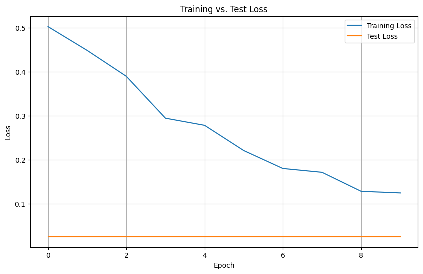
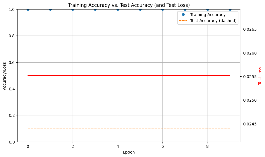
Train-Test Losses Graph of Resnet 50
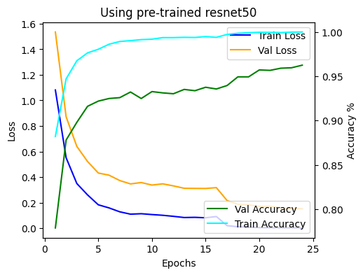
ResNet 50 model Graph
Train-Test Accuracy Graph of VGG 16
Train-Test Losses Graph of VGG16
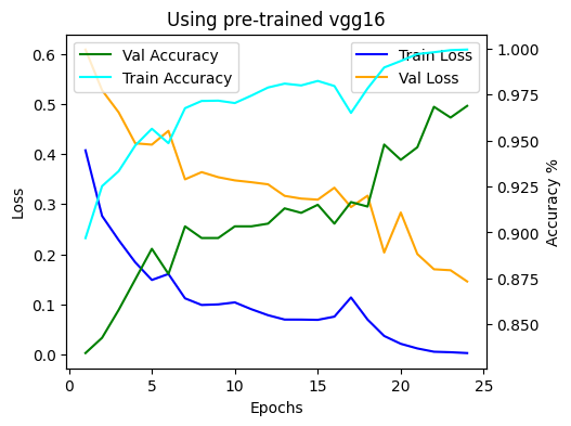
VGG 16 model Graph
After Visualising VGG 16 and ResNet 50 we can say that ResNet 50 performers better than VGG 16 in terms of accuracy.