Real time optimized KMP Algorithm for Pattern Searching

In the article, we have already discussed the KMP algorithm for pattern searching. In this article, a real-time optimized KMP algorithm is discussed. From the previous article, it is known that KMP(a.k.a. Knuth-Morris-Pratt) algorithm preprocesses the pattern P and constructs a failure function F(also called as lps[]) to store the length of the longest suffix of the sub-pattern P[1..l], which is also a prefix of P, for l = 0 to m-1. Note that the sub-pattern starts at index 1 because a suffix can be the string itself. After a mismatched occurred at index P[j], we update j to F[j-1]. The original KMP Algorithm has the runtime complexity of O(M + N) and auxiliary space O(M), where N is the size of the input text and M is the size of the pattern. Preprocessing step costs O(M) time. It is hard to achieve runtime complexity better than that but we are still able to eliminate some inefficient shifts. Inefficiencies of the original KMP algorithm: Consider the following case by using the original KMP algorithm:

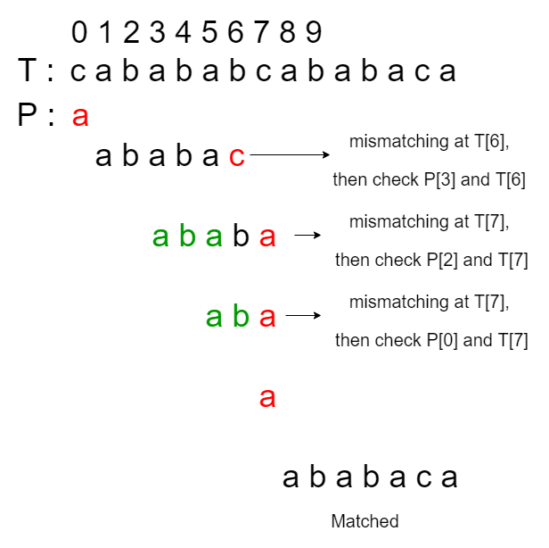
Input: T = “cabababcababaca”, P = “ababaca” Output: Found at index 8

The longest proper prefix or lps[] for the above test case is {0, 0, 1, 2, 3, 0, 1}. Lets assume that the red color represents a mismatch occurs, green color represents the checking we skipped. Therefore, the searching process according to the original KMP algorithm occurs as follows: One thing which can be noticed is that in the third, fourth, and fifth matching, the mismatch occurs at the same location, T[7]. If we can skip the fourth and fifth matching, then the original KMP algorithm can further be optimised to answer the real-time queries. Real-time Optimization: The term real-time in this case can be interpreted as checking each character in the text T at most once. Our goal in this case is to shift the pattern properly (just like KMP algorithm does), but no need to check the mismatched character again. That is, for the same above example, the optimized KMP algorithm should work in the following way:

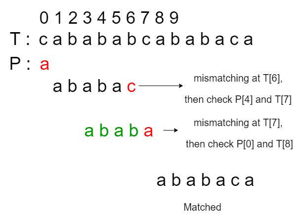
Approach: One way to achieve the goal is to modify the preprocessing process.

• Let K be the size of the letters of the pattern P. We will construct a failure table to contain K failure functions(i.e. lps[]).
• Each failure function in the failure table is mapped to a character(key in the failure table) in the alphabet of the pattern P.
• Recall that the original failure function F[l] (or lps[]) stores the length of the longest suffix of P[1..l], which is also a prefix of P, for l = 0 to m-1, where m is the size of the pattern.
• If a mismatched occurs at T[i] and P[j], the new value of j would be updated to F[j-1] and the counter ‘i’ would be unchanged.
• In our new failure table FT[][], if a failure function F’ is mapped with a character c, F'[l] should store the length of the longest suffix of P[1..l] + c (‘+’ represents appending), which is also a prefix of P, for l = 0 to m-1.
• The intuition is to make proper shifts but also depending on the mismatched character. Here the character c, which is also a key in the failure table, is our “guess” about the mismatched character in the text T.
• That is, if the mismatched character is c, how should we shift the pattern properly? Since we are constructing the failure table in the preprocessing step, we have to make enough guesses about the mismatched character.
• Hence, the number of lps[]’s in the failure table equals to the size of the alphabet of the pattern, and each value, the failure function, should be different with respect to the key, a character in P.
• Assume we have already constructed the desired failure table. Let FT[][] be the failure table, T be the text, P be the pattern.
• Then, in the matching process, if a mismatch occurs at T[i] and P[j] (i.e. T[i] != P[j]):
  1. If T[i] is a character in P, j will be updated to FT[T[i]][j-1], ‘i‘ will be updated to ‘i + 1‘. We are doing this since we are guaranteed that T[i] is matched or skipped.
  2. If T[i] is not a character, ‘j’ will be updated to 0, ‘i’ will be updated to ‘i + 1’.
• Note that if a mismatching does not occur, the behaviour is exactly the same as the original KMP algorithm.

Constructing Failure Table:

• To construct the failure table FT[][], we will need the failure function F(or lps[]) from the original KMP algorithm.
• Since F[l] tells us the length of the longest suffix of the sub-pattern P[1..l], which is also a prefix of P, the values stored in the failure table is one step beyond it.
• That is, for any key t in the failure table FT[][], the values stored in FT[t] is a failure function that satisfies for the character ‘t’ and FT[t][l] stores the length of the longest suffix of a sub-pattern P[1..l] + t(‘+’ means append), which is also a prefix of P, for l from 0 to m-1.
• F[l] has already guaranteed that P[0..F[l]-1] is the longest suffix of the sub-pattern P[1..l], so we will need to check if P[F[l]] is t.
• If true, then we can assign FT[t][l] to be F[l] + 1, as we are guaranteed that P[0..F[l]] is the longest suffix of the sub-pattern P[1..l] + t.
• If false, that indicates P[F[l]] is not t. That is, we fail the matching at character P[F[l]] with the character t, but P[0..F[l]-1] matches a suffix of P[1..l].
• By borrowing the idea from KMP algorithm, just like how we compute the failure function in original KMP algorithm, if the mismatch occurs at P[F[l]] with mismatched character t, we would like to update the next matching starting at FT[t][F[l]-1].
• That is, we use the idea of the KMP algorithm to compute the failure table. Notice that F[l] – 1 is always less than l, so when we are computing FT[t][l], FT[t][F[l] – 1] is ready for us already.
• One special case is that if F[l] is 0 and P[F[l]] is not t, F[l] – 1 has a value of -1, in this case, we will update FT[t][l] to 0. (i.e. there is no suffix of P[1..l] + t exists such that it is a prefix of P.)
• As a conclusion of failure table construction, when we are computing FT[t][l], for any key t and l from 0 to m-1, we will check:

If P[F[l]] is t,
  if yes:
    FT[t][l] <- F[l] + 1;
  if no: 
    check if F[l] is 0,
      if yes:
        FT[t][l] <- 0;
      if no:
        FT[t][l] <- FT[t][F[t] - 1];

• The new preprocessing step has a running time complexity of O(, where is the alphabet set of pattern P, M is the size of P.
• The whole modified KMP algorithm has a running time complexity of O(). The auxiliary space usage of O().
• The running time and space usage look like “worse” than the original KMP algorithm. However, if we are searching for the same pattern in multiple texts or the alphabet set of the pattern is small, as the preprocessing step only needs to be done once and each character in the text will be compared at most once (real-time). So, it is more efficient than the original KMP algorithm and good in practice.

The space complexity is also O(n) because the failure table takes up O(n) space, and the failure function takes up O(n) space as well.