R Shiny Examples

Shiny is an R package that allows us to build interactive web applications directly from the R Programming Language. It bridges the gap between data analysis in R and web development, enabling us to create interactive dashboards.

Basic Structure of Shiny

The UI component defines the layout and appearance of the application, while the server logic dictates how the app responds to user input and generates output.

Suppose we're building a house. In Shiny, our "house" is our app, and it has two main parts: the outside (what people see) and the inside (how things work).

1. The Outside (UI): This is like the outside of our house - what people see when they look at it. In Shiny, it's called the User Interface (UI). It's where we decide what buttons, sliders, text boxes, and other stuff our app will have and how it will look.
2. The Inside (Server): Just like a house has a bunch of wires and pipes behind the walls that make things work, our app has a "brain" called the Server. This is where all the calculations and actions happen. When someone clicks a button or changes a value, the Server reacts and decides what to do next.

UI and Server Components

User Interface (UI)

The User Interface defines the layout, structure, and visual elements of the application that users interact with. It encompasses everything visible to the user, from buttons and input fields to plots and output displays.

Examples of UI Elements:

• Input Fields: Text inputs, sliders, dropdown menus.
• Action Elements: Buttons, checkboxes, radio buttons.
• Output Elements: Plots, data tables, text outputs.

It allowing us to design and customize the appearance of their applications without delving into web development languages like HTML or CSS.

Server Logic

The Server component is where the computational and reactive aspects of the application reside. It consists of R code that responds to user inputs, processes data, and generates dynamic outputs in real-time.

1. Reactive Expressions: Functions that automatically update when their inputs change. They are used to compute intermediate values or perform calculations based on user input.

Syntax:

reactive_expr <- reactive({
  input_val <- input$numInput
  computed_val <- input_val * 2
  return(computed_val)
})

2. Reactive Outputs: Output elements in the UI that are dynamically updated based on changes in reactive expressions or other inputs.

Syntax:

output$plot <- renderPlot({
  input_val <- input$numSlider
  plot(x = seq(1, input_val), y = seq(1, input_val), type = "l")
})

3.Reactive Dependencies: The connections between reactive expressions, inputs, and outputs that define the flow of data and interactions within the application.

Syntax:

observeEvent(input$actionBtn, {
  output$txtOutput <- renderText({
    req(input$txtInput)  # Ensures input is not NULL
    return(paste("You entered:", input$txtInput))
  })
})

Through reactive programming, the Server component ensures that the application remains responsive and adapts to user actions without the need for manual intervention.

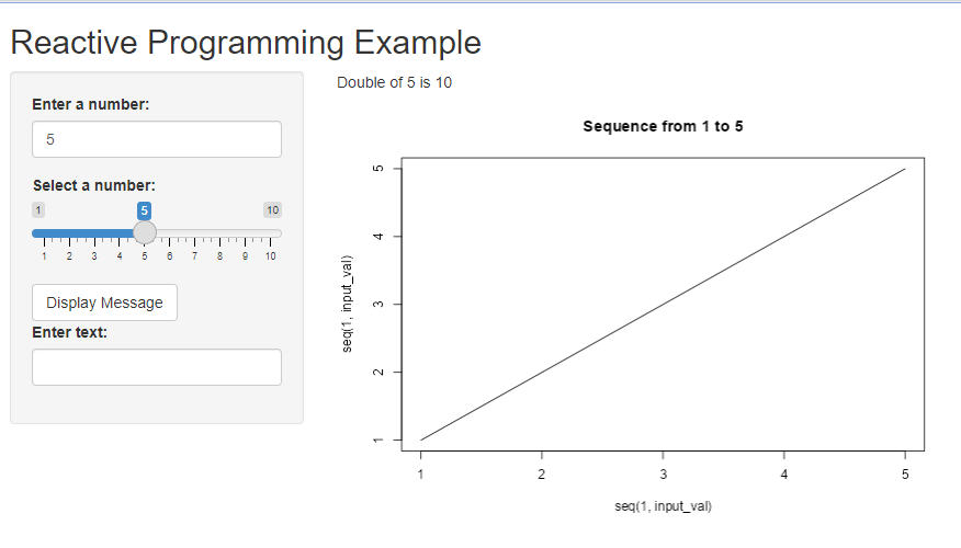
Users input a number, and the app immediately doubles it and displays the result.

• They can select a number on the slider, and the app generates a plot showing a sequence of numbers from 1 to the selected value.
• Users can enter text, and when they click the "Display Message" button, the app shows the entered text.

R

library(shiny)

# Define UI
ui <- fluidPage(
  titlePanel("Reactive Programming Example"),
  sidebarLayout(
    sidebarPanel(
      numericInput("numInput", "Enter a number:", value = 5),
      sliderInput("numSlider", "Select a number:", min = 1, max = 10, value = 5),
      actionButton("actionBtn", "Display Message"),
      textInput("txtInput", "Enter text:")
    ),
    mainPanel(
      textOutput("doubleOutput"),
      plotOutput("plot"),
      textOutput("messageOutput")
    )
  )
)

# Define Server logic
server <- function(input, output, session) {
  
  # Reactive expression to double the numeric input
  output$doubleOutput <- renderText({
    input_val <- input$numInput
    computed_val <- input_val * 2
    paste("Double of", input_val, "is", computed_val)
  })
  
  # Reactive plot output based on the slider value
  output$plot <- renderPlot({
    input_val <- input$numSlider
    plot(x = seq(1, input_val), y = seq(1, input_val), type = "l",
         main = paste("Sequence from 1 to", input_val))
  })
  
  # Observer for button click event
  observeEvent(input$actionBtn, {
    output$messageOutput <- renderText({
      req(input$txtInput)  # Ensures input is not NULL
      paste("You entered:", input$txtInput)
    })
  })
}

# Run the application
shinyApp(ui = ui, server = server)

Output:

R Shiny

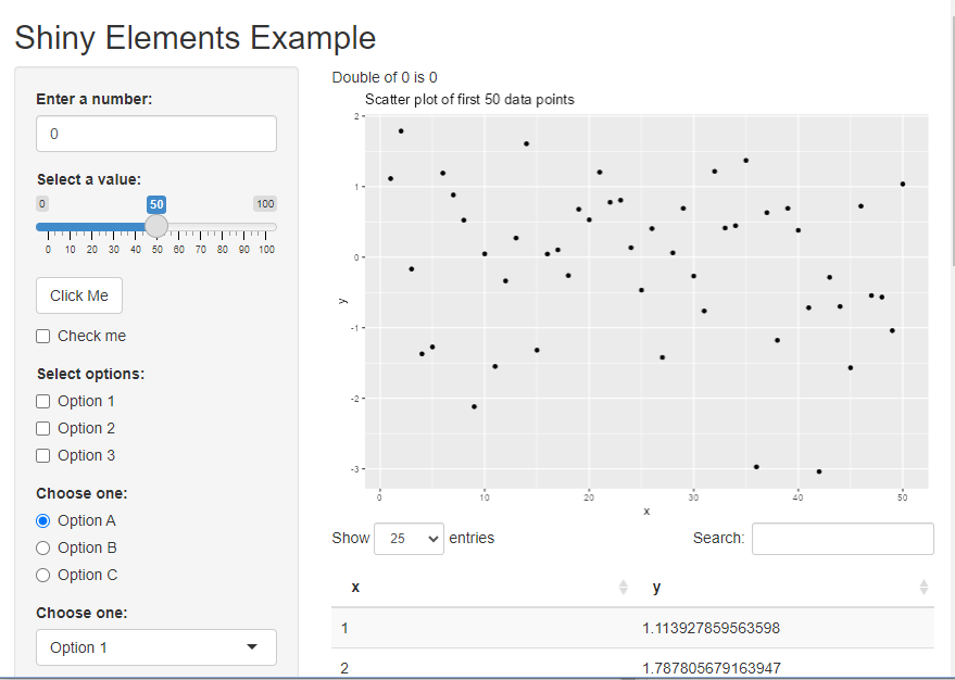
Shiny Elements

1. Sliders: Sliders let users pick a value by sliding a knob along a track. Great for selecting ranges or adjusting parameters.

Syntax:

sliderInput(inputId = "numSlider", label = "Select a value:", min = 0, max = 100, value = 50)

2. Text Inputs: Users can type text or numbers into these boxes. Useful for entering specific values or search terms.

Text Input Syntax:

textInput(inputId = "txtInput", label = "Enter text:")

Numeric Input Syntax:

numericInput(inputId = "numInput", label = "Enter a number:", value = 0)

3. Buttons: Clickable buttons trigger actions when pressed, like submitting a form or updating a plot.

Syntax:

actionButton(inputId = "actionBtn", label = "Click Me")

4. Checkboxes: Checkboxes allow users to select one or more options from a list. Handy for filtering data or making multiple selections.

Single Checkbox Syntax:

checkboxInput(inputId = "singleCheckbox", label = "Check me")

Multiple Checkbox Syntax:

checkboxGroupInput(inputId = "multiCheckbox", label = "Select options:", choices = c("Option 1", "Option 2", "Option 3"))

5. Radio Buttons: Radio buttons let users choose only one option from a list. Good for mutually exclusive choices.

Syntax:

radioButtons(inputId, label, choices, selected = NULL, inline = FALSE)

6.Dropdown Menus: Dropdown menus present a list of options, and users can select one. Useful for conserving space and organizing choices.

Syntax:

selectInput(inputId, label, choices, selected = NULL, multiple = FALSE)

7.Text Outputs: These elements display text or numbers dynamically. They're often used to show results, status messages, or instructions.

Syntax:

textOutput(outputId)

8. Plots: Shiny can create interactive plots using packages like ggplot2 or Plotly. Users can zoom, pan, and hover to explore data visually.

Syntax:

plotOutput(outputId = "plot")

9.Data Tables: Shiny can display tables of data that users can sort, filter, and paginate. Useful for exploring datasets.

Syntax:

dataTableOutput(outputId = "table")

R

library(shiny)
library(ggplot2)

# Sample dataset
data <- data.frame(
  x = seq(1, 100),
  y = rnorm(100)
)

# Define UI
ui <- fluidPage(
  titlePanel("Shiny Elements Example"),
  sidebarLayout(
    sidebarPanel(
      numericInput("numInput", "Enter a number:", value = 0),
      sliderInput("numSlider", "Select a value:", min = 0, max = 100, value = 50),
      actionButton("actionBtn", "Click Me"),
      checkboxInput("singleCheckbox", "Check me"),
      checkboxGroupInput("multiCheckbox", "Select options:", 
                         choices = c("Option 1", "Option 2", "Option 3")),
      radioButtons("radioBtn", "Choose one:", 
                   choices = c("Option A", "Option B", "Option C"), selected = NULL),
      selectInput("dropdownMenu", "Choose one:", 
                  choices = c("Option 1", "Option 2", "Option 3"), selected = NULL),
      textInput("txtInput", "Enter text:")
    ),
    mainPanel(
      textOutput("doubleOutput"),
      plotOutput("plot"),
      textOutput("messageOutput"),
      dataTableOutput("table")
    )
  )
)

# Define Server logic
server <- function(input, output, session) {
  
  # Reactive expression to double the numeric input
  output$doubleOutput <- renderText({
    input_val <- input$numInput
    computed_val <- input_val * 2
    paste("Double of", input_val, "is", computed_val)
  })
  
  # Reactive plot output based on the slider value
  output$plot <- renderPlot({
    input_val <- input$numSlider
    ggplot(data[1:input_val, ], aes(x = x, y = y)) +
      geom_point() +
      labs(title = paste("Scatter plot of first", input_val, "data points"))
  })
  
  # Observer for button click event
  observeEvent(input$actionBtn, {
    output$messageOutput <- renderText({
      req(input$txtInput)  # Ensures input is not NULL
      paste("You entered:", input$txtInput)
    })
  })
  
  # Render a sample data table
  output$table <- renderDataTable({
    data
  })
}

# Run the application
shinyApp(ui = ui, server = server)

Output:

R Shiny

Layout Management

Layout management is simply the arrangement and organization of visual elements within a user interface (UI). It involves deciding where to put buttons, text fields, images, and other elements to make them easy to find and use. In Shiny, layout management means using functions like fluidPage() or navbarPage() to structure our app's layout. These functions help us decide where to place different parts of our app, like the main content, sidebars, or navigation bars.

1. fluidPage()

fluidPage() creates a fluid layout that adjusts to the size of the browser window.

• It's the most commonly used layout function in Shiny applications.
• All UI components placed within fluidPage() will resize dynamically based on the available screen space.

Synatx:

ui <- fluidPage(
  titlePanel("My Shiny App"),
  sidebarLayout(
    sidebarPanel(
      # Sidebar content
    ),
    mainPanel(
      # Main content
    )
  )
)

2.navbarPage()

navbarPage() creates a layout with a navigation bar at the top, allowing users to navigate between different pages or tabs. It's useful for organizing content into multiple sections or views within the same application.

Synatx:

ui <- navbarPage(
  "My App",
  tabPanel("Tab 1", 
    # Content for Tab 1
  ),
  tabPanel("Tab 2", 
    # Content for Tab 2
  )
)

3. sidebarLayout()

sidebarLayout() divides the page into a sidebar and a main panel. It's often used when we want to display controls or additional information in a sidebar alongside the main content.

Syntax:-

ui <- fluidPage(
  titlePanel("My Shiny App"),
  sidebarLayout(
    sidebarPanel(
      # Sidebar content
    ),
    mainPanel(
      # Main content
    )
  )
)

Interactive plotting

Interactive plotting allows users to engage with data visualizations in real-time. Unlike static plots, interactive plots enable users to:-

1. Interact: Users can hover over data points, zoom in/out, pan across the plot, and select specific data for detailed examination.
2. Update Dynamically: Plots respond instantly to user actions or changes in data, providing immediate feedback.
3. Customize: Users can personalize plots by adjusting colors, labels, axes, and annotations to suit their preferences.
4. Integrate: Interactive plots can be seamlessly integrated into web applications, dashboards, and analytics platforms for enhanced data exploration and analysis.

Creating interactive plots with libraries like ggplot2 and plotly in Shiny allows us to enhance data visualization and engage users with dynamic visualizations.

Using ggplot2

• First, create a ggplot object as you normally would in R.
• Use renderPlot() in the server function to render the ggplot object.
• Place plotOutput() in the UI function to define where the plot will be displayed.

Syntax:

# UI
ui <- fluidPage(
  plotOutput("ggplot")
)

# Server
server <- function(input, output) {
  output$ggplot <- renderPlot({
    ggplot(data = iris, aes(x = Sepal.Length, y = Sepal.Width, color = Species)) +
      geom_point()
  })
}

2. Using plotly

• Create a plotly object using functions provided by the plotly package.
• Use renderPlotly() in the server function to render the plotly object.
• Place plotlyOutput() in the UI function to define where the plot will be displayed.

Syntax:

# UI
ui <- fluidPage(
  plotlyOutput("plotly")
)

# Server
server <- function(input, output) {
  output$plotly <- renderPlotly({
    plot_ly(data = iris, x = ~Sepal.Length, y = ~Sepal.Width, color = ~Species, type = "scatter", mode = "markers")
  })
}

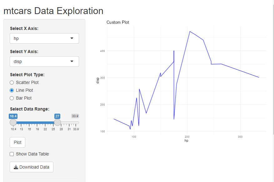
Creating Interactive Shiny App

1. Select X and Y Axes: Users can choose the variables for the X and Y axes from dropdown menus.
2. Select Plot Type: They can select between Scatter Plot, Line Plot, and Bar Plot using radio buttons.
3. Select Data Range: Specify a range of data based on the "mpg" variable using sliders.
4. Show Data Table: Users can toggle the display of a data table showing the filtered dataset using a checkbox.
5. Download Data: Download the displayed data table as a CSV file.
6. Additional Options: Users can customize the appearance of the plot by selecting point shapes and colors, inputting a custom plot title, and updating the plot with the selected customizations using an action button.
7. Custom CSS Styles: The app includes custom CSS styles to enhance the appearance of the buttons.

R

library(shiny)
library(ggplot2)
library(DT)

# Define UI
ui <- fluidPage(
  titlePanel("mtcars Data Exploration"),
  
  sidebarLayout(
    sidebarPanel(
      selectInput("x_axis", "Select X Axis:", 
                  choices = c("mpg", "cyl", "disp", "hp", "drat", "wt", "qsec", "vs", 
                              "am", "gear", "carb")),
      selectInput("y_axis", "Select Y Axis:", 
                  choices = c("mpg", "cyl", "disp", "hp", "drat", "wt", "qsec", "vs", 
                              "am", "gear", "carb")),
      radioButtons("plot_type", "Select Plot Type:", 
                   choices = c("Scatter Plot", "Line Plot", "Bar Plot"), 
                   selected = "Scatter Plot"),
      sliderInput("data_range", "Select Data Range:",
                  min = min(mtcars$mpg), max = max(mtcars$mpg),
                  value = c(min(mtcars$mpg), max(mtcars$mpg)), step = 1),
      actionButton("plotBtn", "Plot"),
      checkboxInput("showTable", "Show Data Table", value = FALSE),
      downloadButton("downloadData", "Download Data"),
      hr(),
      # Additional options
      selectInput("point_shape", "Select Point Shape:", 
                  choices = c(0, 1, 2, 3, 4, 5, 6, 7, 8, 9, 10, 11, 12, 13, 14, 15, 
                              16, 17, 18, 19, 20)),
      selectInput("point_color", "Select Point Color:", 
                  choices = c("red", "blue", "green", "yellow", "orange", "purple", 
                              "black")),
      textInput("plot_title", "Plot Title:", value = "Custom Plot"),
      actionButton("updateBtn", "Update Plot")
    ),
    
    mainPanel(
      plotOutput("plot"),
      DTOutput("dataTable")
    )
  ),
  # Add custom CSS styles
  tags$head(tags$style(HTML("
    .btn-primary { background-color: #FF5733; border-color: #FF5733; }
    .btn-primary:hover { background-color: #FF7851; border-color: #FF7851; }
    .btn-primary:focus { background-color: #FF7851; border-color: #FF7851; }
    .btn-primary:active { background-color: #FF7851; border-color: #FF7851; }
  ")))
)

# Define server logic
server <- function(input, output) {
  # Reactive expression to filter data based on selected data range
  filteredData <- reactive({
    subset(mtcars, mpg >= input$data_range[1] & mpg <= input$data_range[2])
  })
  
  # Generate plot based on selected options
  output$plot <- renderPlot({
    plot_data <- filteredData()
    if (input$plot_type == "Scatter Plot") {
      ggplot(plot_data, aes_string(x = input$x_axis, y = input$y_axis)) +
        geom_point(shape = input$point_shape, color = input$point_color) +
        labs(title = input$plot_title,
             x = input$x_axis, y = input$y_axis) +
        theme_minimal()
    } else if (input$plot_type == "Line Plot") {
      ggplot(plot_data, aes_string(x = input$x_axis, y = input$y_axis)) +
        geom_line(color = input$point_color) +
        labs(title = input$plot_title,
             x = input$x_axis, y = input$y_axis) +
        theme_minimal()
    } else {
      ggplot(plot_data, aes_string(x = input$x_axis)) +
        geom_bar(fill = input$point_color) +
        labs(title = input$plot_title,
             x = input$x_axis, y = "Count") +
        theme_minimal()
    }
  })
  
  # Show/hide data table based on checkbox
  output$dataTable <- renderDT({
    if (input$showTable) {
      filteredData()
    } else {
      NULL
    }
  })
  
  # Download data table as CSV
  output$downloadData <- downloadHandler(
    filename = function() {
      paste("mtcars_data", ".csv", sep = "")
    },
    content = function(file) {
      write.csv(filteredData(), file, row.names = FALSE)
    }
  )
}

# Run the application
shinyApp(ui = ui, server = server)

Output:

R Shiny

Conclusion

Shiny apps provide a user-friendly and interactive way to explore data and create data-driven applications. By combining the power of R programming with web development, Shiny allows users to build dynamic and customizable interfaces without requiring extensive coding knowledge. With its wide range of input widgets, reactive programming capabilities, and seamless integration with popular R packages like ggplot2 and DT, Shiny enables users to create engaging and informative visualizations and dashboards. Whether for data analysis, reporting, or sharing insights, Shiny offers a versatile platform for data exploration and communication.