Support Vector Machines (SVMs) are a powerful machine learning technique excelling at classifying data. Imagine a scenario where you have a collection of red and blue marbles, and your goal is to draw a clear dividing line to separate them. SVMs achieve this by not just creating a separation, but by finding the optimal separation boundary, ensuring the maximum distance between the line and the closest marbles from each color. This wide separation, known as the margin, enhances the model's ability to handle unseen data. In this tutorial, we will construct decision boundary for breast cancer problem.
Core Concepts of SVMs
- Maximizing the Margin: The core principle of Support Vector Machines (SVMs) lies in maximizing the margin, the space between the decision boundary (think of a fence) and the closest data points (imagine houses) from each class. A wider margin translates to a more robust model, better equipped to classify new data points accurately. Just like a wider road between houses reduces traffic accidents, a larger margin reduces classification errors.
- Support Vectors: These are the most crucial data points, acting like pillars in construction. They are the closest points to the decision boundary and directly influence its placement. If these points shift, the entire boundary needs to be adjusted, highlighting their significance in shaping the classification model.
- Kernel Trick: Real-world data often isn't perfectly separable by a straight line. The kernel trick tackles this challenge by essentially lifting the data points into a higher-dimensional space where a clear separation becomes possible. Imagine sorting objects on a flat table. The kernel trick lifts them into a 3D space for sorting, before bringing them back down to the original space with a potentially curved or more complex decision boundary. This empowers SVMs to handle non-linear data effectively.
SVMs are particularly valuable for classification tasks. Let's look at a real-world example: classifying breast cancer tumors as malignant or benign. Here, the data points represent features extracted from mammograms, and the SVM's job is to learn the optimal decision boundary to distinguish between the two classes.
By analyzing features like cell size and shape, the SVM can create a separation line that effectively categorizes tumors. The wider the margin between this line and the closest malignant and benign data points (support vectors), the more confident the SVM can be in its classifications.
SVM Decision Boundary Construction with Linear Kernel
In this section, we focus on the construction of decision boundaries using SVMs with a linear kernel. The linear kernel represents a fundamental approach where the decision boundary is a hyperplane in the feature space. This straightforward yet robust method is particularly effective when the data is linearly separable, meaning classes can be separated by a straight line or plane.
Mathematically, the linear kernel [Tex]K(x_i, x_j)[/Tex] between two feature vectors [Tex]x_i[/Tex]and [Tex]x_j[/Tex]is calculated as:
[Tex]K(x_i,x_j)=x_{i}^{T}x_j [/Tex]
Here, [Tex]x_{i}^{T}[/Tex]denotes the transpose of the feature vector [Tex]x_i[/Tex], and [Tex]x_{i}^{T} x_j[/Tex] represents the dot product between the two vectors. This formulation captures the linear relationship between features and serves as the basis for constructing decision boundaries using SVMs with a linear kernel.
Implementation: SVM Decision Boundary Construction using Linear Kernel
In the following code, have loaded the breast cancer dataset and create a SVM classifier using Linear Kernel.
import numpy as np
import matplotlib.pyplot as plt
from sklearn import datasets
from sklearn import svm
from sklearn.model_selection import train_test_split
from sklearn.preprocessing import StandardScaler
from sklearn.metrics import confusion_matrix, ConfusionMatrixDisplay

# Load the Breast Cancer dataset
cancer = datasets.load_breast_cancer()
X = cancer.data
y = cancer.target

# We will use only the first two features for visualization purposes
X = X[:, :2]

# Preprocess the dataset
scaler = StandardScaler()
X_scaled = scaler.fit_transform(X)

# Split the data into a training set and a test set
X_train, X_test, y_train, y_test = train_test_split(X_scaled, y, test_size=0.3, random_state=42)

# Create an SVM classifier
clf = svm.SVC(kernel='linear', C=1.0)
clf.fit(X_train, y_train)
In this step, we we will be visualizing the decision boundaries of a Support Vector Machine (SVM) classifier trained on the Breast Cancer dataset.
A mesh grid is created to cover the entire range of feature values in the dataset. The h variable determines the step size of the grid. x_min, x_max, y_min, and y_max represent the minimum and maximum values of the features in the dataset. np.meshgrid() is then used to create coordinate matrices (xx and yy) from the ranges of x and y values.
# Create a mesh to plot
h = .02  # step size in the mesh
x_min, x_max = X_scaled[:, 0].min() - 1, X_scaled[:, 0].max() + 1
y_min, y_max = X_scaled[:, 1].min() - 1, X_scaled[:, 1].max() + 1
xx, yy = np.meshgrid(np.arange(x_min, x_max, h), np.arange(y_min, y_max, h))
In this part, the SVM classifier (clf) predicts the class labels for each point in the mesh grid. np.c_[] is used to concatenate the coordinate matrices xx and yy into a single matrix of feature values for prediction. The ravel() function is used to flatten the matrices into 1D arrays, which can be fed into the classifier. The predicted labels (Z) are then reshaped to match the shape of the mesh grid (xx.shape).
# Predict class labels for each point in the mesh
Z = clf.predict(np.c_[xx.ravel(), yy.ravel()])
Z = Z.reshape(xx.shape)
# Put the result into a color plot
plt.contourf(xx, yy, Z, cmap=plt.cm.coolwarm, alpha=0.8)
Here, you can find the complete code for visualizing the boundaries.
plt.figure(figsize=(12, 6))
# Create a mesh to plot
h = .02  # step size in the mesh
x_min, x_max = X_scaled[:, 0].min() - 1, X_scaled[:, 0].max() + 1
y_min, y_max = X_scaled[:, 1].min() - 1, X_scaled[:, 1].max() + 1
xx, yy = np.meshgrid(np.arange(x_min, x_max, h), np.arange(y_min, y_max, h))

# Predict class labels for each point in the mesh
Z = clf.predict(np.c_[xx.ravel(), yy.ravel()])
Z = Z.reshape(xx.shape)
# Put the result into a color plot
plt.contourf(xx, yy, Z, cmap=plt.cm.coolwarm, alpha=0.8)

# Plot also the training points
plt.scatter(X_train[:, 0], X_train[:, 1], c=y_train, cmap=plt.cm.coolwarm, edgecolors='k')
plt.xlabel('Feature 1')
plt.ylabel('Feature 2')
plt.xlim(xx.min(), xx.max())
plt.ylim(yy.min(), yy.max())
plt.title('SVM Decision Surface using Breast Cancer dataset')
plt.show()
Output:
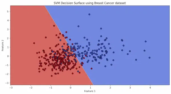
The decision boundary, depicted by the line separating the red and blue areas, discriminates between malignant and benign cases based on the first two features of the dataset.
# Evaluate the model using the test set
accuracy = clf.score(X_test, y_test)
print(f'The model accuracy on the test set is: {accuracy * 100:.2f}%')

# Confusion Matrix
cm = confusion_matrix(y_test, clf.predict(X_test))
disp = ConfusionMatrixDisplay(confusion_matrix=cm, display_labels=cancer.target_names)
disp.plot(cmap=plt.cm.Blues)
plt.show()
Output:
The model accuracy on the test set is: 90.06%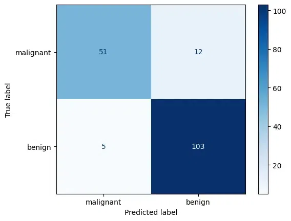
The confusion matrix quantifies the model's predictions, with the majority of true labels correctly matched with the predicted labels, indicating a high degree of accuracy.
SVM Decision Boundary Construction with RBF Kernel
In this section, we focus on the construction of decision boundaries using SVMs with the RBF kernel. Unlike the linear kernel, which assumes a linear relationship between features, the RBF kernel is capable of capturing complex, non-linear relationships in the data. This makes it particularly suitable for scenarios where classes are not easily separable by a straight line or plane in the feature space.
The RBF kernel, also known as the Gaussian kernel, computes the similarity between feature vectors in the original feature space by measuring the distance between them in a high-dimensional space. Mathematically, the RBF kernel [Tex]K(x_i, x_j)[/Tex] between two feature vectors [Tex]x_i[/Tex] and [Tex]x_j[/Tex] is calculated as:
[Tex]K(x_i,x_j)=exp(−γ⋅∣∣x_i−x_j∣∣^{2})[/Tex]
Here, [Tex]∣∣x_i−x_j∣∣^2[/Tex] represents the squared Euclidean distance between the feature vectors [Tex]x_i[/Tex] and [Tex]x_j[/Tex], and [Tex]\gamma[/Tex] is a parameter that controls the influence of each training example on the decision boundary. The exponential term [Tex]exp(−γ⋅∣∣xi−xj∣∣^2)[/Tex] ensures that closer points have a higher similarity, while farther points have a lower similarity.
Implementation: SVM Decision Boundary Construction using RBF Kernel
Now, will be creating decision boundaries using RBF kernel using the following code:
# Create an SVM classifier
clf = svm.SVC(kernel='rbf', C=1.0)
clf.fit(X_train, y_train)
To visualize the boundaries using the same code, we used before for visualizing the SVM boundaries for linear kernel.
plt.figure(figsize=(12, 6))
# Create a mesh to plot
h = .02  # step size in the mesh
x_min, x_max = X_scaled[:, 0].min() - 1, X_scaled[:, 0].max() + 1
y_min, y_max = X_scaled[:, 1].min() - 1, X_scaled[:, 1].max() + 1
xx, yy = np.meshgrid(np.arange(x_min, x_max, h), np.arange(y_min, y_max, h))

# Predict class labels for each point in the mesh
Z = clf.predict(np.c_[xx.ravel(), yy.ravel()])
Z = Z.reshape(xx.shape)
# Put the result into a color plot
plt.contourf(xx, yy, Z, cmap=plt.cm.coolwarm, alpha=0.8)

# Plot also the training points
plt.scatter(X_train[:, 0], X_train[:, 1], c=y_train, cmap=plt.cm.coolwarm, edgecolors='k')
plt.xlabel('Feature 1')
plt.ylabel('Feature 2')
plt.xlim(xx.min(), xx.max())
plt.ylim(yy.min(), yy.max())
plt.title('SVM Decision Surface using Breast Cancer dataset')
plt.show()
Output:

We can observe, that the decision boundary produced by SVMs with an RBF kernel is non-linear.
Now, let's evaluated the model.
# Evaluate the model using the test set
accuracy = clf.score(X_test, y_test)
print(f'The model accuracy on the test set is: {accuracy * 100:.2f}%')

# Confusion Matrix
cm = confusion_matrix(y_test, clf.predict(X_test))
disp = ConfusionMatrixDisplay(confusion_matrix=cm, display_labels=cancer.target_names)
disp.plot(cmap=plt.cm.Blues)
plt.show()
Output:
The model accuracy on the test set is: 90.64%.png)
Conclusion
SVMs offer a robust approach to classification by focusing on maximizing the margin between classes. Their ability to handle non-linear data through the kernel trick makes them even more versatile. By understanding the core concepts of margins, support vectors, and the kernel trick, you can gain better understanding at how SVMs excel at creating optimal boundaries in the world of machine learning.