Gaussian Distribution In Machine Learning

The Gaussian distribution, also known as the normal distribution, plays a fundamental role in machine learning. It is a key concept used to model the distribution of real-valued random variables and is essential for understanding various statistical methods and algorithms.

Gaussian Distribution

In machine learning, the Gaussian distribution, is also known as the normal distribution. It is a continuous probability distribution function that is symmetrical at the mean, and the majority of data falls within one standard deviation of the mean. It is characterized by its bell-shaped curve.

Gaussian Distribution Formula

The PDF (probability density function) of the Gaussian distribution is given by the formula:

[Tex]f(x) = \frac{1}{\sigma \sqrt{2\pi}} \exp \left( -\frac{(x - \mu)^2}{2\sigma^2} \right) [/Tex]

where:

• x represents the Variable
• μ represents the Mean
• σ represents the Standard Deviation
• e represents the base of the Natural Logarithm.

Gaussian Distribution Curve

The curve is symmetric and bell-shaped, and it mathematically represents the probability distribution of a continuous random variable. The Gaussian distribution is characterized by two parameters: the mean (μ) and the standard deviation (σ), which determine the location and the spread of the curve.

• The standard deviations are used to subdivide the area under the normal curve. Each subdivided section defines the percentage of data, which falls into the specific region of a graph.
• Analysis : A smaller standard deviation results in a narrower and taller bell curve, indicating that data points are clustered closely around the mean. Conversely, a larger standard deviation leads to a wider and shorter bell curve, suggesting that data points are more spread out from the mean.
• The Empirical Rule, also known as the 68-95-99.7 rule, quantifies the proportion of data falling within certain intervals around the mean in a normal distribution. It provides a quick way to estimate the spread of data without performing detailed calculations.

• Within one standard deviation of the mean (Mean ± 1 SD), approximately 68% of the data is expected to fall.
• Within two standard deviations of the mean (Mean ± 2 SD), approximately 95% of the data is expected to fall.
• Within three standard deviations of the mean (Mean ± 3 SD), approximately 99.7% of the data is expected to fall.

Gaussian Distribution Table

• A Gaussian distribution table, also known as a standard normal distribution table or z-table, is a tabulated form that provides values of the cumulative distribution function (CDF) for the standard normal distribution.
• The standard normal distribution has a mean(central value) of 0 and a standard deviation of 1.
• Normally , the table consists of two columns namely Z-value and their Cumulative probability . Z-value is the number of standard deviations away from the mean. It ranges from negative infinity to positive infinity.
• Cumulative probability represents the probability that a standard normal random variable is less than or equal to the corresponding z-value.

Note:

• Columns = value of z ranging from -3.4 to 3.4, with increments of 0.1.
• Rows = percentile value ranging from 0.00 to 0.09, with increments of 0.01.

Z-Value	0	0.01	0.02	0.03	0.04	0.05	0.06	0.07	0.08	0.09
0	0	0.004	0.008	0.012	0.016	0.0199	0.0239	0.0279	0.0319	0.0359
0.1	0.0398	0.0438	0.0478	0.0517	0.0557	0.0596	0.0636	0.0675	0.0714	0.0753
0.2	0.0793	0.0832	0.0871	0.091	0.0948	0.0987	0.1026	0.1064	0.1103	0.1141
0.3	0.1179	0.1217	0.1255	0.1293	0.1331	0.1368	0.1406	0.1443	0.148	0.1517
0.4	0.1554	0.1591	0.1628	0.1664	0.17	0.1736	0.1772	0.1808	0.1844	0.1879
0.5	0.1915	0.195	0.1985	0.2019	0.2054	0.2088	0.2123	0.2157	0.219	0.2224
0.6	0.2257	0.2291	0.2324	0.2357	0.2389	0.2422	0.2454	0.2486	0.2517	0.2549
0.7	0.258	0.2611	0.2642	0.2673	0.2704	0.2734	0.2764	0.2794	0.2823	0.2852
0.8	0.2881	0.291	0.2939	0.2967	0.2995	0.3023	0.3051	0.3078	0.3106	0.3133
0.9	0.3159	0.3186	0.3212	0.3238	0.3264	0.3289	0.3315	0.334	0.3365	0.3389
1	0.3413	0.3438	0.3461	0.3485	0.3508	0.3531	0.3554	0.3577	0.3599	0.3621
1.1	0.3643	0.3665	0.3686	0.3708	0.3729	0.3749	0.377	0.379	0.381	0.383
1.2	0.3849	0.3869	0.3888	0.3907	0.3925	0.3944	0.3962	0.398	0.3997	0.4015
1.3	0.4032	0.4049	0.4066	0.4082	0.4099	0.4115	0.4131	0.4147	0.4162	0.4177
1.4	0.4192	0.4207	0.4222	0.4236	0.4251	0.4265	0.4279	0.4292	0.4306	0.4319
1.5	0.4332	0.4345	0.4357	0.437	0.4382	0.4394	0.4406	0.4418	0.4429	0.4441
1.6	0.4452	0.4463	0.4474	0.4484	0.4495	0.4505	0.4515	0.4525	0.4535	0.4545
1.7	0.4554	0.4564	0.4573	0.4582	0.4591	0.4599	0.4608	0.4616	0.4625	0.4633
1.8	0.4641	0.4649	0.4656	0.4664	0.4671	0.4678	0.4686	0.4693	0.4699	0.4706
1.9	0.4713	0.4719	0.4726	0.4732	0.4738	0.4744	0.475	0.4756	0.4761	0.4767
2	0.4772	0.4778	0.4783	0.4788	0.4793	0.4798	0.4803	0.4808	0.4812	0.4817

The Z score table is often used in statistical calculations and hypothesis testing to determine probabilities associated with specific z-values.

For example , z-value of 1.96 in the table then the cumulative probability to be approximately 0.975 , we can infer that approximately 97.5% of the area under the standard normal curve lies to the left of z = 1.96.

Properties of Gaussian Distribution

Some of the important properties are

• The Gaussian distribution must be symmetric around its mean with same probability density on both sides of mean.
• The sum of many independent, identically distributed random variables converges to a Gaussian distribution.
• When you estimate the mean and variance of a Gaussian distribution from a set of data, the maximum likelihood estimators provide the most accurate estimates compared to other distributions.
• In linear transformations, if X follows a Gaussian distribution, then aX+b also follows a Gaussian distribution for constants a and b. This property makes the Gaussian distribution robust and convenient for modeling various real-world phenomena that involve linear transformations.
• In multiple dimensions, the Gaussian distribution extends naturally. It describes how multiple variables can be jointly Gaussian, meaning that any linear combination of these variables also follows a Gaussian distribution. This property is valuable for modeling complex systems with multiple interacting variables.

Machine Learning Methods that uses Gaussian Distribution

• Likelihood Modeling: In algorithms, such as linear regression, logistic regression, and Gaussian mixture models, it is often assumed that the observed data is generated from a Gaussian distribution. It simplifies the model and allows for efficient parameter estimation.
• Bayesian Inference: In Bayesian machine learning, the Gaussian distribution is commonly used as a prior distribution over model parameters. This prior distribution reflects about the parameters before observing any data and is updated to a posterior distribution using Bayes' theorem.
• Clustering: Gaussian mixture models (GMMs) can model complex data distributions and are often used in image segmentation and data compression.
• Anomaly Detection: Gaussian distribution is often used in anomaly detection algorithms, where the goal is to identify rare events or outliers in the data. Anomalies are detected based on the likelihood of the data under the Gaussian distribution.
• Dimensionality Reduction: Principal Component Analysis (PCA), it finds the directions of maximum variance in the data, which correspond to the principal components.
• Kernel Methods: Gaussian kernel is commonly used in kernelized machine learning algorithms, such as Support Vector Machines (SVMs) and Gaussian Processes (GPs), to define the similarity between data points.
  

Implementation of Gaussian Distribution in Machine Learning

Consider the famous Iris dataset consists of 150 samples of iris flowers, each with four features: sepal length, sepal width, petal length, and petal width. We can examine the distribution of one of these features, such as sepal length, using a histogram to see if it approximately follows a Gaussian distribution.

• x = np.linspace(np.min(sepal_length), np.max(sepal_length), 100) : the np.linspace function is used to create an array of 100 evenly spaced numbers between the minimum and maximum values of the sepal length feature (sepal_length). This array is used to plot the Gaussian distribution curve.

Python3

from sklearn.datasets import load_iris
import matplotlib.pyplot as plt
import numpy as np

# Load the Iris dataset
iris = load_iris()
sepal_length = iris.data[:, 0]  # Extract sepal length (feature at index 0)

mu, std = np.mean(sepal_length), np.std(sepal_length)
x = np.linspace(np.min(sepal_length), np.max(sepal_length), 100)
y = (1 / (std * np.sqrt(2 * np.pi))) * np.exp(-0.5 * ((x - mu) / std)**2)

plt.figure(figsize=(8, 6))
plt.hist(sepal_length, bins=20, color='skyblue', edgecolor='black', alpha=0.7, density=True)
plt.plot(x, y, color='red', label='Gaussian Fit')
plt.xlabel('Sepal Length (cm)')
plt.ylabel('Density')
plt.title('Distribution of Sepal Length in Iris Dataset with Gaussian Fit')
plt.legend()
plt.show()

Output:

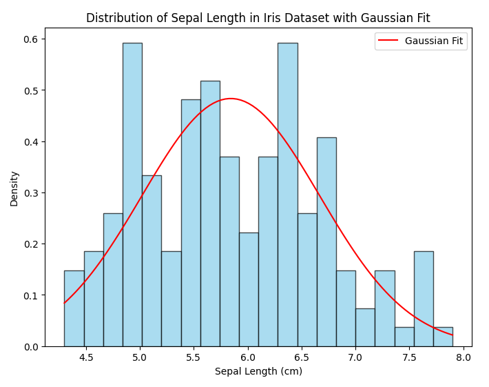
FIGURE 1

• Central Tendency: The peak of the distribution (mean) suggests that the most common sepal length among the iris flowers in the dataset is around 5.8 centimeters.
• Variability: The spread of the distribution (standard deviation) indicates how much the sepal lengths vary from the mean. A larger standard deviation would imply more variability in sepal lengths among the iris flowers.
• Normality: The distribution roughly follows a bell-shaped curve, which is characteristic of a normal (Gaussian) distribution. This suggests that sepal lengths in the Iris dataset may be normally distributed.
• Outliers: The presence of outliers, particularly on the right tail of the distribution, indicates that there are some iris flowers with unusually long sepal lengths compared to the rest of the dataset. These outliers could be due to measurement errors or represent a distinct subgroup of iris flowers.

The stability of Gaussian distributions under linear combinations facilitates analytical solutions for understanding the behavior of random variables and making predictions based on data making it a cornerstone in statistical modeling and analysis.