Non-linear regression is used to fit relationships between variables that are beyond the capability of linear regression. It can fit intricate relationships like exponential, logarithmic and polynomial relationships. Caret, a package in R, offers a simple interface to develop and compare machine learning models, including non-linear regressions.
Caret Package in R
The Caret package is widely used in R for building and evaluating machine learning models. It provides a unified interface to various machine learning algorithms, including linear and non-linear models, decision trees, random forests, support vector machines and neural networks. Some of the key features of the Caret package include:
- Data cleaning: Methods such as centering, scaling, feature selection and outlier detection.
- Cross-validation: Provides several cross-validation techniques, including k-fold and leave-one-out.
- Model tuning: Uses grid search, random search and Bayesian optimization to perform hyperparameter tuning.
- Processing in parallel: Accelerates model training and testing by exploiting multiple cores.
Non-linear regression using Caret in R
To illustrate non-linear regression using the Caret package, we will use the Iris dataset built into R. We will forecast the Petal.Length variable using Sepal.Length as a predictor in a non-linear model and assess its performance with 10-fold cross-validation
Step 1: Install and Load Required Libraries
We shall require the Caret and ggplot2 libraries for building the model and visualization, respectively.
# Load the required libraries
library(caret)
library(ggplot2)
Step 2: Load the Dataset
The data we'll use in our example is then loaded. Here, we're using R's native "Iris" dataset. This might be replaced for any other dataset of your preference.
# Load the dataset (Iris dataset)
data(iris)
Step 3: Define the Non-Linear Regression Model:
We will specify the non-linear regression model with the nls() function (non-linear least squares). The formula is a quadratic relationship between Petal.Length and Sepal.Length.
# Define the non-linear regression model
model <- nls(Petal.Length ~ a*Sepal.Length^2 + b*Sepal.Length + c,
             data = iris,
             start = list(a = 0.01,
                          b = 0.1, c = 1))

# Define a function to predict
# petal length from sepal length
predict_petallength <- function(sepal_length) {
  predict(model, newdata = data.frame(Sepal.Length = sepal_length))
}
Step 4: Train and Evaluate the Model Using Caret
We'll make use of the caret package's train() function to do 10-fold cross-validation. The model will be trained on the lm (linear regression) method and we'll check its performance
# Train and evaluate the model using the caret package
train_control <- trainControl(method = "cv", number = 10)
model_caret <- train(Petal.Length ~ predict_petallength(Sepal.Length),
                     data = iris, method = "lm",
                     trControl = train_control)

summary(model_caret)
Output:
Call:
lm(formula = .outcome ~ ., data = dat)
Residuals:
Min 1Q Median 3Q Max
-2.6751 -0.5138 0.1218 0.5356 2.6287
Coefficients:
Estimate Std. Error t value Pr(>|t|)
(Intercept) -1.654e-08 1.788e-01 0.00 1
`predict_petallength(Sepal.Length)` 1.000e+00 4.399e-02 22.73 <2e-16 ***
---
Signif. codes: 0 ‘***’ 0.001 ‘**’ 0.01 ‘*’ 0.05 ‘.’ 0.1 ‘ ’ 1
Residual standard error: 0.8357 on 148 degrees of freedom
Multiple R-squared: 0.7774, Adjusted R-squared: 0.7759
F-statistic: 516.8 on 1 and 148 DF, p-value: < 2.2e-16
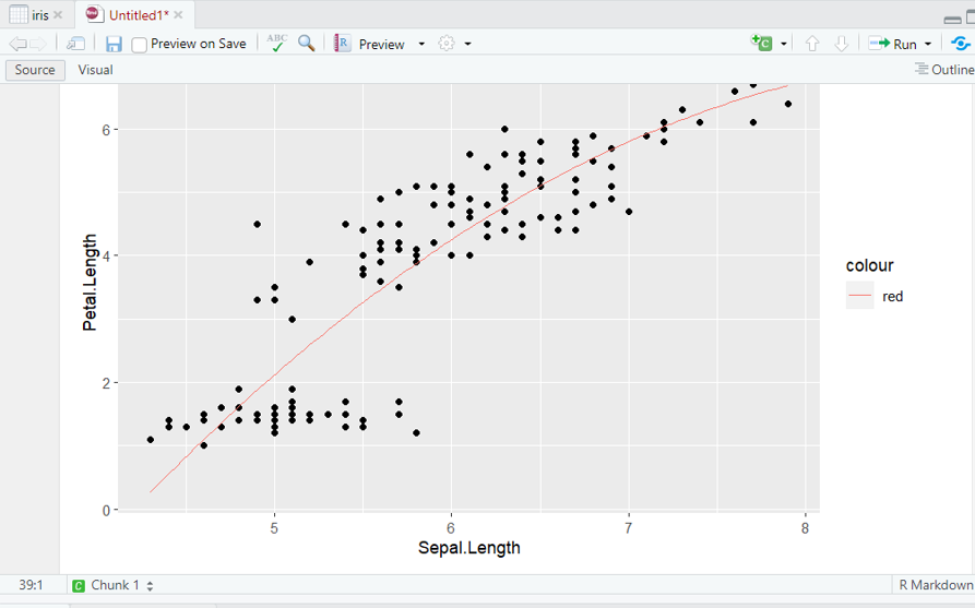
Step 5: Visualize the Model
Lastly, we will plot the relationship between Sepal.Length and Petal.Length with the non-linear regression line superimposed on a scatterplot.
# Plot the results
library(ggplot2)

ggplot(iris, aes(Sepal.Length, Petal.Length))
    + geom_point()
    + stat_function(fun = predict_petallength,
                    color = "red", size = 1)
Output: