XLOOKUP Function in Excel With Examples

XLOOKUP Function helps us to search value in a horizontal or vertical dataset and return the relative value in some other row or column. In this article, we will look at the XLOOKUP Function in Excel. XLOOKUP is a modern replacement for functions like HLOOKUP, VLOOKUP, and LOOKUP. XLOOKUP supports approximate and exact matching, wildcards for partial matches, and lookups in horizontal or vertical ranges. XLOOKUP can be performed in Microsoft 365.

What is XLOOKUP in Excel

XLOOKUP in Excel is a newer and more versatile way to find and retrieve data. It’s easier to use than older lookup functions and can search in any direction (vertical or horizontal). XLOOKUP handles errors, supports wildcards for partial matches, and can return arrays of values. It’s great for working with large datasets and simplifies many common tasks.

XLOOKUP Vs VLOOKUP in Excel

XLOOKUP and VLOOKUP are Excel functions used for finding information in a table, but they have differences:

XLOOKUP

• More versatile, handles both vertical and horizontal lookups.
• Easier syntax, with no need to specify column numbers.
• Built-in error handling with custom error messages.
• Supports wildcards for flexible searches.
• Can return arrays of values.
• Works well with large datasets and dynamic arrays.

VLOOKUP

• Primarily for vertical lookups.
• Requires specifying column index, which can be cumbersome.
• Basic error handling using the “IFERROR” function.
• Defaults to exact matches; requires extra steps for approximate matches.
• Returns a single value, not suitable for multiple matches.
• In essence, XLOOKUP is more user-friendly and powerful, especially for complex tasks, while VLOOKUP is simpler but has limitations.

How to Use XLOOKUP in Excel

XLOOKUP Function Syntax

=XLOOKUP(lookup_value, lookup_array, return_array,  [if _not_found], [match_mode], [search_mode])

Parameter:

• lookup_value: The value which we want to search
• lookup_array: The range in which we want to search
• if_not_found (Optional): The text which we want to return if the value is not found
• match_mode (Optional): Here we can specify the type of match we want.

Match Type	Behavior
0 (default)	Here it will look for an exact match
-1	If we do not get the exact match then it will return the next smaller item.
1	If we do not get the exact match then it will return the next larger item.
2	It will do partial matching using (* or ~)

• search_mode (Optional): where we can specify how the function should look up the value.

Search mode	Behavior
1(default)	It will search the values first.
-1	It will search the values in reverse from last.
2	It will perform a binary search and data needs to be sorted in ascending order.
-2	It will perform a binary search and data needs to be sorted in descending order.

In simple language :
=XLOOKUP(search for this value, in this range, and Return a match from this range).

Below are some examples of the XLOOKUP.

How to Enable XLOOKUP in Excel

To access the XLOOKUP function in Excel, you need to be using a version of Excel that supports it.

Excel 365

XLOOKUP is included in Excel 365, which is a subscription-based version of Excel that receives regular updates and new features.

Excel 2019

XLOOKUP was introduced in Excel 2019, which is a one-time purchase version of Excel. However, it might not be available in older versions of Excel, such as Excel 2016 or earlier.

XLOOKUP Function Examples

Below are some examples through which the XLOOKUP function will be easily understandable.

Exact Match

This function in XLOOKUP is by default. 

Follow the below steps to Lookup a value:

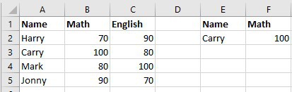
Step 1: Format your data.

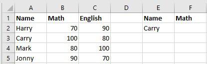
Now, if we want to get the math marks of Carry then follow the next step

Step 2: We will enter =XLOOKUP(E2, A2:A5, B2:B5) in the F2 cell to get the marks of carrying.

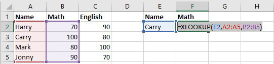
Then we will get the math marks for carry.

Approximate Match

Let’s consider the below example for Approximate match mode.

Formula used is : =XLOOKUP(lookup value, in this range, Return a value from this range, -1)

Here -1 will return the approximate value which is smaller than the lookup value. 

Note: The user can also use 1 instead of -1 to return a value larger than the lookup value. The XLOOKUP function can also work for Unsorted data.

Left Lookup

Using INDEX and MATCH in Excel left lookup can be performed but to make it simple and quick you can also use the XLOOKUP function. This XLOOKUP function is used to search the values which are on the left side of the searched values.

The formula used: = XLOOKUP(Search for this value, from this range, and return the output from this range)

Here the output we are looking for will be from the left side of the column.

Multiple Values

Follow the below steps to look up the values of the entire row:

Step 1: Format your data.

Now, if we want to get the Math and English marks for carrying then follow the next step

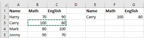
Step 2: We will enter =XLOOKUP(E2,A2:A5,B2:C5) in F2 cell.

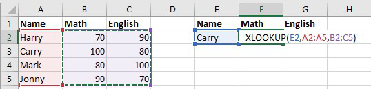
Then we will get the Math and English marks.

Nested XLOOKUP function

Follow the below steps to use nested XLOOKUP functions:

Step 1: Format your data.

Now, if we want to get the math marks of Carry by two-way lookup then follow the next step.

Step 2: We will enter =XLOOKUP(F1,B1:C1,XLOOKUP(E2,A2:A5,B2:C5)) in F2 cell.

Here, XLOOKUP(E2, A2:A5, B2:C5) is{100,80} which is an array mark of Carry. In the outer XLOOKUP formula, we are looking for the subject name which is in the F1 cell and the lookup array is B1:C1.

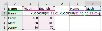
Then we will get the math marks of carry.

Not Found

Follow the below steps when the LOOKUP function returns the Not Found message:

Step 1: Format your data.

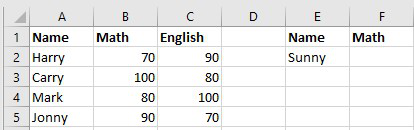
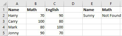
If we want the marks of Sunny who is not in the dataset

Step 2: We will enter =XLOOKUP(E2,A2:A5,B2:B5,”Not Found”) in F2 cell.

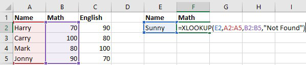
Then it will show Not Found.

SUM function

Follow the below steps to find the sum of a range:

Step 1: Format your data.

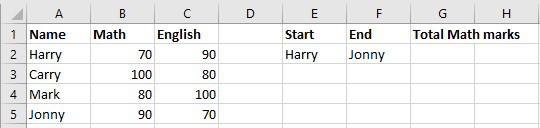
If we want the total math marks from Harry to Jonny then do the next step

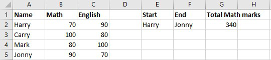
Step 2: We will enter =SUM(XLOOKUP(E2,A2:A5,B1:B6):XLOOKUP(F2,A2:A5,B1:B6)) in G2 cell this simply means =SUM($B$2:$B$5).

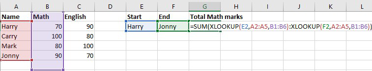
Then we will get the sum.

Horizontal Lookup

Step 1: Format your data.

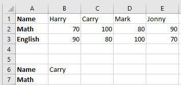
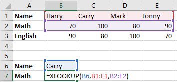
Now, if we want to get the math marks of Carry then follow the next step

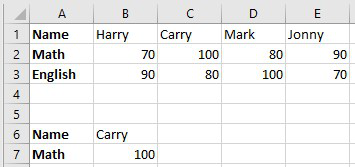
Step 2: We will enter =XLOOKUP(B6,B1:E1,B2:E2) in B7 cell.

Then we will get the math marks of Carry

Last Match

By default, the XLOOKUP Function performs a top-to-bottom search. But if the user wants to change this order and search for the bottom to top then the formula should be: =XLOOKUP(Search for the value, in this range, return the output from this range, -1)

Note: -1 in this formula should be the 6th parameter) 

FAQs on XLOOKUP Function in Excel

Q1: Why XLOOKUP formula is better?

Answer:

XLOOKUP is better in the following ways:

• Cool to type
• Gives Reference as output.
• XLOOKUP makes the most used formula in Excel easy to use.

Q2: What are the optional parameters in the XLOOKUP formula?

Answer:

By default, Excel has only three parameters which are as follows:

In simple language :

=XLOOKUP(what you want to look, lookup list, result list)

Other than these three parameters you can also use the 4th, 5th, and 6th parameters to specify more about your LOOKUP value.

4th Parameter (If not found):  This resolves the error problem.

For example :

 =XLOOKUP(“Ravi”,Student[Student name],Student[total[],”Value not found”)

It will return Value not found instead of error if the lookup value is not available in the search column (student name).

5th Parameter: Match mode or type. This tells Excel how you want your match.

By default (0): Exact Match 

(-1): Exact match or next smaller value.

(1): Exact match or next Larger value.

(2): Wild card character match. 

6th Parameter: Match Direction 

 By default, the direction is top-down. Use this if you want to search from bottom to top. 

Q3: What is the issue with XLOOKUP function?

Answer:

The issue with the XLOOKUP function is that it is not backward compatible. That means if you use XLOOKUP in a particular file and open it in a version that does not have XLOOKUP function then it will show an error. 

Q4: How to copy the XLOOKUP formula in Multiple Cells?

Answer:

While copying an XLOOKUP formula to multiple cells, Lock the LOOKUP or return ranges with Absolut cell reference to prevent them from changing.