Word Embeddings are numeric representations of words in a lower-dimensional space, capturing semantic and syntactic information. They play a vital role in Natural Language Processing (NLP) tasks. This article explores traditional and neural approaches, such as TF-IDF, Word2Vec, and GloVe, offering insights into their advantages and disadvantages. Understanding the importance of pre-trained word embeddings, providing a comprehensive understanding of their applications in various NLP scenarios.
What is Word Embedding in NLP?
Word Embedding is an approach for representing words and documents. Word Embedding or Word Vector is a numeric vector input that represents a word in a lower-dimensional space. It allows words with similar meanings to have a similar representation.
Word Embeddings are a method of extracting features out of text so that we can input those features into a machine learning model to work with text data. They try to preserve syntactical and semantic information. The methods such as Bag of Words (BOW), CountVectorizer and TFIDF rely on the word count in a sentence but do not save any syntactical or semantic information. In these algorithms, the size of the vector is the number of elements in the vocabulary. We can get a sparse matrix if most of the elements are zero. Large input vectors will mean a huge number of weights which will result in high computation required for training. Word Embeddings give a solution to these problems.
Need for Word Embedding?
- To reduce dimensionality
- To use a word to predict the words around it.
- Inter-word semantics must be captured.
How are Word Embeddings used?
- They are used as input to machine learning models.
Take the words —-> Give their numeric representation —-> Use in training or inference. - To represent or visualize any underlying patterns of usage in the corpus that was used to train them.
Let’s take an example to understand how word vector is generated by taking emotions which are most frequently used in certain conditions and transform each emoji into a vector and the conditions will be our features.

In a similar way, we can create word vectors for different words as well on the basis of given features. The words with similar vectors are most likely to have the same meaning or are used to convey the same sentiment.
Approaches for Text Representation
1. Traditional Approach
The conventional method involves compiling a list of distinct terms and giving each one a unique integer value, or id. and after that, insert each word’s distinct id into the sentence. Every vocabulary word is handled as a feature in this instance. Thus, a large vocabulary will result in an extremely large feature size. Common traditional methods include:
1.1. One-Hot Encoding
One-hot encoding is a simple method for representing words in natural language processing (NLP). In this encoding scheme, each word in the vocabulary is represented as a unique vector, where the dimensionality of the vector is equal to the size of the vocabulary. The vector has all elements set to 0, except for the element corresponding to the index of the word in the vocabulary, which is set to 1.
Python3
def one_hot_encode(text):
words = text.split()
vocabulary = set(words)
word_to_index = {word: i for i, word in enumerate(vocabulary)}
one_hot_encoded = []
for word in words:
one_hot_vector = [0] * len(vocabulary)
one_hot_vector[word_to_index[word]] = 1
one_hot_encoded.append(one_hot_vector)
return one_hot_encoded, word_to_index, vocabulary
example_text = "cat in the hat dog on the mat bird in the tree"
one_hot_encoded, word_to_index, vocabulary = one_hot_encode(example_text)
print("Vocabulary:", vocabulary)
print("Word to Index Mapping:", word_to_index)
print("One-Hot Encoded Matrix:")
for word, encoding in zip(example_text.split(), one_hot_encoded):
print(f"{word}: {encoding}")
|
Output:
Vocabulary: {'mat', 'the', 'bird', 'hat', 'on', 'in', 'cat', 'tree', 'dog'}
Word to Index Mapping: {'mat': 0, 'the': 1, 'bird': 2, 'hat': 3, 'on': 4, 'in': 5, 'cat': 6, 'tree': 7, 'dog': 8}
One-Hot Encoded Matrix:
cat: [0, 0, 0, 0, 0, 0, 1, 0, 0]
in: [0, 0, 0, 0, 0, 1, 0, 0, 0]
the: [0, 1, 0, 0, 0, 0, 0, 0, 0]
hat: [0, 0, 0, 1, 0, 0, 0, 0, 0]
dog: [0, 0, 0, 0, 0, 0, 0, 0, 1]
on: [0, 0, 0, 0, 1, 0, 0, 0, 0]
the: [0, 1, 0, 0, 0, 0, 0, 0, 0]
mat: [1, 0, 0, 0, 0, 0, 0, 0, 0]
bird: [0, 0, 1, 0, 0, 0, 0, 0, 0]
in: [0, 0, 0, 0, 0, 1, 0, 0, 0]
the: [0, 1, 0, 0, 0, 0, 0, 0, 0]
tree: [0, 0, 0, 0, 0, 0, 0, 1, 0]
While one-hot encoding is a simple and intuitive method for representing words in NLP, it has several disadvantages, which may limit its effectiveness in certain applications.
- One-hot encoding results in high-dimensional vectors, making it computationally expensive and memory-intensive, especially with large vocabularies.
- It does not capture semantic relationships between words; each word is treated as an isolated entity without considering its meaning or context.
- It is restricted to the vocabulary seen during training, making it unsuitable for handling out-of-vocabulary words.
1.2. Bag of Word (Bow)
Bag-of-Words (BoW) is a text representation technique that represents a document as an unordered set of words and their respective frequencies. It discards the word order and captures the frequency of each word in the document, creating a vector representation.
Python3
from sklearn.feature_extraction.text import CountVectorizer
documents = ["This is the first document.",
"This document is the second document.",
"And this is the third one.",
"Is this the first document?"]
vectorizer = CountVectorizer()
X = vectorizer.fit_transform(documents)
feature_names = vectorizer.get_feature_names_out()
print("Bag-of-Words Matrix:")
print(X.toarray())
print("Vocabulary (Feature Names):", feature_names)
|
Output:
Bag-of-Words Matrix:
[[0 1 1 1 0 0 1 0 1]
 [0 2 0 1 0 1 1 0 1]
 [1 0 0 1 1 0 1 1 1]
 [0 1 1 1 0 0 1 0 1]]
Vocabulary (Feature Names): ['and' 'document' 'first' 'is' 'one' 'second' 'the' 'third' 'this']
While BoW is a simple and interpretable representation, below disadvantages highlight its limitations in capturing certain aspects of language structure and semantics:
- BoW ignores the order of words in the document, leading to a loss of sequential information and context making it less effective for tasks where word order is crucial, such as in natural language understanding.
- BoW representations are often sparse, with many elements being zero resulting in increased memory requirements and computational inefficiency, especially when dealing with large datasets.
1.3. Term frequency-inverse document frequency (TF-IDF)
Term Frequency-Inverse Document Frequency, commonly known as TF-IDF, is a numerical statistic that reflects the importance of a word in a document relative to a collection of documents (corpus). It is widely used in natural language processing and information retrieval to evaluate the significance of a term within a specific document in a larger corpus. TF-IDF consists of two components:
- Term Frequency (TF): Term Frequency measures how often a term (word) appears in a document. It is calculated using the formula:

- Inverse Document Frequency (IDF): Inverse Document Frequency measures the importance of a term across a collection of documents. It is calculated using the formula:

The TF-IDF score for a term t in a document d is then given by multiplying the TF and IDF values:

The higher the TF-IDF score for a term in a document, the more important that term is to that document within the context of the entire corpus. This weighting scheme helps in identifying and extracting relevant information from a large collection of documents, and it is commonly used in text mining, information retrieval, and document clustering.
Let’s Implement Term Frequency-Inverse Document Frequency (TF-IDF) using python with the scikit-learn library. It begins by defining a set of sample documents. The TfidfVectorizer is employed to transform these documents into a TF-IDF matrix. The code then extracts and prints the TF-IDF values for each word in each document. This statistical measure helps assess the importance of words in a document relative to their frequency across a collection of documents, aiding in information retrieval and text analysis tasks.
Python3
from sklearn.feature_extraction.text import TfidfVectorizer
documents = [
"The quick brown fox jumps over the lazy dog.",
"A journey of a thousand miles begins with a single step.",
]
vectorizer = TfidfVectorizer()
tfidf_matrix = vectorizer.fit_transform(documents)
feature_names = vectorizer.get_feature_names_out()
tfidf_values = {}
for doc_index, doc in enumerate(documents):
feature_index = tfidf_matrix[doc_index, :].nonzero()[1]
tfidf_doc_values = zip(feature_index, [tfidf_matrix[doc_index, x] for x in feature_index])
tfidf_values[doc_index] = {feature_names[i]: value for i, value in tfidf_doc_values}
for doc_index, values in tfidf_values.items():
print(f"Document {doc_index + 1}:")
for word, tfidf_value in values.items():
print(f"{word}: {tfidf_value}")
print("\n")
|
Output:
Document 1:
dog: 0.3404110310756642
lazy: 0.3404110310756642
over: 0.3404110310756642
jumps: 0.3404110310756642
fox: 0.3404110310756642
brown: 0.3404110310756642
quick: 0.3404110310756642
the: 0.43455990318254417
Document 2:
step: 0.3535533905932738
single: 0.3535533905932738
with: 0.3535533905932738
begins: 0.3535533905932738
miles: 0.3535533905932738
thousand: 0.3535533905932738
of: 0.3535533905932738
journey: 0.3535533905932738
TF-IDF is a widely used technique in information retrieval and text mining, but its limitations should be considered, especially when dealing with tasks that require a deeper understanding of language semantics. For example:
- TF-IDF treats words as independent entities and doesn’t consider semantic relationships between them. This limitation hinders its ability to capture contextual information and word meanings.
- Sensitivity to Document Length: Longer documents tend to have higher overall term frequencies, potentially biasing TF-IDF towards longer documents.
2. Neural Approach
2.1. Word2Vec
Word2Vec is a neural approach for generating word embeddings. It belongs to the family of neural word embedding techniques and specifically falls under the category of distributed representation models. It is a popular technique in natural language processing (NLP) that is used to represent words as continuous vector spaces. Developed by a team at Google, Word2Vec aims to capture the semantic relationships between words by mapping them to high-dimensional vectors. The underlying idea is that words with similar meanings should have similar vector representations. In Word2Vec every word is assigned a vector. We start with either a random vector or one-hot vector.
There are two neural embedding methods for Word2Vec, Continuous Bag of Words (CBOW) and Skip-gram.
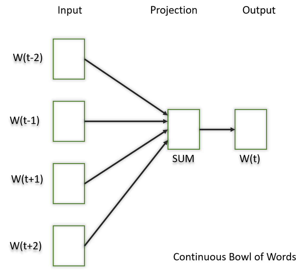
2.2. Continuous Bag of Words(CBOW)
Continuous Bag of Words (CBOW) is a type of neural network architecture used in the Word2Vec model. The primary objective of CBOW is to predict a target word based on its context, which consists of the surrounding words in a given window. Given a sequence of words in a context window, the model is trained to predict the target word at the center of the window.
CBOW is a feedforward neural network with a single hidden layer. The input layer represents the context words, and the output layer represents the target word. The hidden layer contains the learned continuous vector representations (word embeddings) of the input words.
The architecture is useful for learning distributed representations of words in a continuous vector space.
The hidden layer contains the continuous vector representations (word embeddings) of the input words.
- The weights between the input layer and the hidden layer are learned during training.
- The dimensionality of the hidden layer represents the size of the word embeddings (the continuous vector space).
Python3
import torch
import torch.nn as nn
import torch.optim as optim
class CBOWModel(nn.Module):
def __init__(self, vocab_size, embed_size):
super(CBOWModel, self).__init__()
self.embeddings = nn.Embedding(vocab_size, embed_size)
self.linear = nn.Linear(embed_size, vocab_size)
def forward(self, context):
context_embeds = self.embeddings(context).sum(dim=1)
output = self.linear(context_embeds)
return output
context_size = 2
raw_text = "word embeddings are awesome"
tokens = raw_text.split()
vocab = set(tokens)
word_to_index = {word: i for i, word in enumerate(vocab)}
data = []
for i in range(2, len(tokens) - 2):
context = [word_to_index[word] for word in tokens[i - 2:i] + tokens[i + 1:i + 3]]
target = word_to_index[tokens[i]]
data.append((torch.tensor(context), torch.tensor(target)))
vocab_size = len(vocab)
embed_size = 10
learning_rate = 0.01
epochs = 100
cbow_model = CBOWModel(vocab_size, embed_size)
criterion = nn.CrossEntropyLoss()
optimizer = optim.SGD(cbow_model.parameters(), lr=learning_rate)
for epoch in range(epochs):
total_loss = 0
for context, target in data:
optimizer.zero_grad()
output = cbow_model(context)
loss = criterion(output.unsqueeze(0), target.unsqueeze(0))
loss.backward()
optimizer.step()
total_loss += loss.item()
print(f"Epoch {epoch + 1}, Loss: {total_loss}")
word_to_lookup = "embeddings"
word_index = word_to_index[word_to_lookup]
embedding = cbow_model.embeddings(torch.tensor([word_index]))
print(f"Embedding for '{word_to_lookup}': {embedding.detach().numpy()}")
|
Output:
Embedding for 'embeddings': [[-2.7053456   2.1384873   0.6417674   1.2882394   0.53470695  0.5651745
   0.64166373 -1.1691749   0.32658175 -0.99961764]]
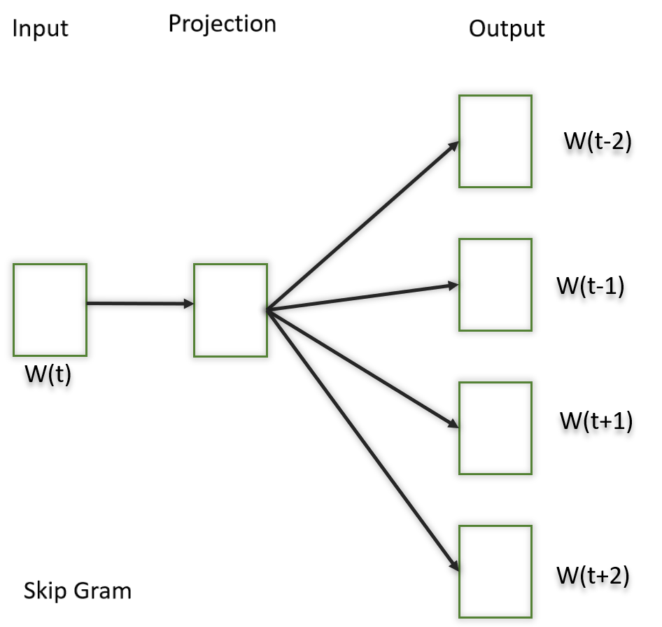
2.3. Skip-Gram
The Skip-Gram model learns distributed representations of words in a continuous vector space. The main objective of Skip-Gram is to predict context words (words surrounding a target word) given a target word. This is the opposite of the Continuous Bag of Words (CBOW) model, where the objective is to predict the target word based on its context. It is shown that this method produces more meaningful embeddings.
After applying the above neural embedding methods we get trained vectors of each word after many iterations through the corpus. These trained vectors preserve syntactical or semantic information and are converted to lower dimensions. The vectors with similar meaning or semantic information are placed close to each other in space.
Let’s understand with a basic example. The python code contains, vector_size parameter that controls the dimensionality of the word vectors, and you can adjust other parameters such as window based on your specific needs.
Note: Word2Vec models can perform better with larger datasets. If you have a large corpus, you might achieve more meaningful word embeddings.
Python3
!pip install gensim
from gensim.models import Word2Vec
from nltk.tokenize import word_tokenize
import nltk
nltk.download('punkt')
sample = "Word embeddings are dense vector representations of words."
tokenized_corpus = word_tokenize(sample.lower())
skipgram_model = Word2Vec(sentences=[tokenized_corpus],
vector_size=100,
window=5,
sg=1,
min_count=1,
workers=4)
skipgram_model.train([tokenized_corpus], total_examples=1, epochs=10)
skipgram_model.save("skipgram_model.model")
loaded_model = Word2Vec.load("skipgram_model.model")
vector_representation = loaded_model.wv['word']
print("Vector representation of 'word':", vector_representation)
|
Output:
Vector representation of 'word': [-9.5800208e-03  8.9437785e-03  4.1664648e-03  9.2367809e-03
  6.6457358e-03  2.9233587e-03  9.8055992e-03 -4.4231843e-03
 -6.8048164e-03  4.2256550e-03  3.7299085e-03 -5.6668529e-03
--------------------------------------------------------------
  2.8835384e-03 -1.5386029e-03  9.9318363e-03  8.3507905e-03
  2.4184163e-03  7.1170190e-03  5.8888551e-03 -5.5787875e-03]
In practice, the choice between CBOW and Skip-gram often depends on the specific characteristics of the data and the task at hand. CBOW might be preferred when training resources are limited, and capturing syntactic information is important. Skip-gram, on the other hand, might be chosen when semantic relationships and the representation of rare words are crucial.
3. Pretrained Word-Embedding
Pre-trained word embeddings are representations of words that are learned from large corpora and are made available for reuse in various natural language processing (NLP) tasks. These embeddings capture semantic relationships between words, allowing the model to understand similarities and relationships between different words in a meaningful way.
3.1. GloVe
GloVe is trained on global word co-occurrence statistics. It leverages the global context to create word embeddings that reflect the overall meaning of words based on their co-occurrence probabilities. this method, we take the corpus and iterate through it and get the co-occurrence of each word with other words in the corpus. We get a co-occurrence matrix through this. The words which occur next to each other get a value of 1, if they are one word apart then 1/2, if two words apart then 1/3 and so on.
Let us take an example to understand how the matrix is created. We have a small corpus:
Corpus:
It is a nice evening.
Good Evening!
Is it a nice evening?
|
| 0 | | | | | |
| 1+1 | 0 | | | | |
| 1/2+1 | 1+1/2 | 0 | | | |
| 1/3+1/2 | 1/2+1/3 | 1+1 | 0 | | |
| 1/4+1/3 | 1/3+1/4 | 1/2+1/2 | 1+1 | 0 | |
| 0 | 0 | 0 | 0 | 1 | 0 |
The upper half of the matrix will be a reflection of the lower half. We can consider a window frame as well to calculate the co-occurrences by shifting the frame till the end of the corpus. This helps gather information about the context in which the word is used.
Initially, the vectors for each word is assigned randomly. Then we take two pairs of vectors and see how close they are to each other in space. If they occur together more often or have a higher value in the co-occurrence matrix and are far apart in space then they are brought close to each other. If they are close to each other but are rarely or not frequently used together then they are moved further apart in space.
After many iterations of the above process, we’ll get a vector space representation that approximates the information from the co-occurrence matrix. The performance of GloVe is better than Word2Vec in terms of both semantic and syntactic capturing.
Python3
from gensim.models import KeyedVectors
from gensim.downloader import load
glove_model = load('glove-wiki-gigaword-50')
word_pairs = [('learn', 'learning'), ('india', 'indian'), ('fame', 'famous')]
for pair in word_pairs:
similarity = glove_model.similarity(pair[0], pair[1])
print(f"Similarity between '{pair[0]}' and '{pair[1]}' using GloVe: {similarity:.3f}")
|
Output:
Similarity between 'learn' and 'learning' using GloVe: 0.802
Similarity between 'india' and 'indian' using GloVe: 0.865
Similarity between 'fame' and 'famous' using GloVe: 0.589
3.2. Fasttext
Developed by Facebook, FastText extends Word2Vec by representing words as bags of character n-grams. This approach is particularly useful for handling out-of-vocabulary words and capturing morphological variations.
Python3
import gensim.downloader as api
fasttext_model = api.load("fasttext-wiki-news-subwords-300")
word_pairs = [('learn', 'learning'), ('india', 'indian'), ('fame', 'famous')]
for pair in word_pairs:
similarity = fasttext_model.similarity(pair[0], pair[1])
print(f"Similarity between '{pair[0]}' and '{pair[1]}' using FastText: {similarity:.3f}")
|
Output:
Similarity between 'learn' and 'learning' using Word2Vec: 0.642
Similarity between 'india' and 'indian' using Word2Vec: 0.708
Similarity between 'fame' and 'famous' using Word2Vec: 0.519
3.3. BERT (Bidirectional Encoder Representations from Transformers)
BERT is a transformer-based model that learns contextualized embeddings for words. It considers the entire context of a word by considering both left and right contexts, resulting in embeddings that capture rich contextual information.
Python3
from transformers import BertTokenizer, BertModel
import torch
model_name = 'bert-base-uncased'
tokenizer = BertTokenizer.from_pretrained(model_name)
model = BertModel.from_pretrained(model_name)
word_pairs = [('learn', 'learning'), ('india', 'indian'), ('fame', 'famous')]
for pair in word_pairs:
tokens = tokenizer(pair, return_tensors='pt')
with torch.no_grad():
outputs = model(**tokens)
cls_embedding = outputs.last_hidden_state[:, 0, :]
similarity = torch.nn.functional.cosine_similarity(cls_embedding[0], cls_embedding[1], dim=0)
print(f"Similarity between '{pair[0]}' and '{pair[1]}' using BERT: {similarity:.3f}")
|
Output:
Similarity between 'learn' and 'learning' using BERT: 0.930
Similarity between 'india' and 'indian' using BERT: 0.957
Similarity between 'fame' and 'famous' using BERT: 0.956
Considerations for Deploying Word Embedding Models
- You need to use the exact same pipeline during deploying your model as were used to create the training data for the word embedding. If you use a different tokenizer or different method of handling white space, punctuation etc. you might end up with incompatible inputs.
- Words in your input that doesn’t have a pre-trained vector. Such words are known as Out of Vocabulary Word(oov). What you can do is replace those words with “UNK” which means unknown and then handle them separately.
- Dimension mis-match: Vectors can be of many lengths. If you train a model with vectors of length say 400 and then try to apply vectors of length 1000 at inference time, you will run into errors. So make sure to use the same dimensions throughout.
Advantages and Disadvantage of Word Embeddings
Advantages
- It is much faster to train than hand build models like WordNet (which uses graph embeddings).
- Almost all modern NLP applications start with an embedding layer.
- It Stores an approximation of meaning.
Disadvantages
- It can be memory intensive.
- It is corpus dependent. Any underlying bias will have an effect on your model.
- It cannot distinguish between homophones. Eg: brake/break, cell/sell, weather/whether etc.
Conclusion
In conclusion, word embedding techniques such as TF-IDF, Word2Vec, and GloVe play a crucial role in natural language processing by representing words in a lower-dimensional space, capturing semantic and syntactic information.
Frequently Asked Questions (FAQs)
1. Does GPT use word embeddings?
GPT uses context-based embeddings rather than traditional word embeddings. It captures word meaning in the context of the entire sentence.
2. What is the difference between Bert and word embeddings?
BERT is contextually aware, considering the entire sentence, while traditional word embeddings, like Word2Vec, treat each word independently.
3. What are the two types of word embedding?
Word embeddings can be broadly evaluated in two categories, intrinsic and extrinsic. For intrinsic evaluation, word embeddings are used to calculate or predict semantic similarity between words, terms, or sentences.
4. How does word vectorization work?
Word vectorization converts words into numerical vectors, capturing semantic relationships. Techniques like TF-IDF, Word2Vec, and GloVe are common.
5. What are the benefits of word embeddings?
Word embeddings offer semantic understanding, capture context, and enhance NLP tasks. They reduce dimensionality, speed up training, and aid in language pattern recognition.
Like Article
Suggest improvement
Share your thoughts in the comments
Please Login to comment...