What are different types of denoising filters in MATLAB?

Digital images are prone to various types of noise that make the quality of the images worst. Image noise is a random variation of brightness or color information in the captured image. Noise is basically the degradation in image signal caused by external sources such as cameras. Images containing multiplicative noise have the characteristic that the brighter the area the noisier it. We shall discuss various denoising filters in order to remove these noises from the digital images. 

Types of filters discussed in this article are listed as:

• Mean filter
• Median filter
• Gaussian filter  
• Wiener filter

Mean Filter

• It is also called as Box Averaging filtering technique.
• It uses a kernel and is based on convolution.
• It calculates the average of all a pixel and its surrounding pixels and the result is assigned to the central pixel.
• It is a very effective technique for the removal of Poisson noise.

Syntax:

 k=rgb2gray(k); // To convert into grayscale: 

 gaussian_noise = imnoise(k, ‘gaussian’, 0, 0.01);

// To create the image corrupted with gaussian noise:

denoised=conv2(noisy_image, mean_filter, ‘same’); 

// To perform the convolution between gaussian_noisy image and mean filter:

To display the image: imtool( image_variable, [ ]);

To create the image corrupted with poisson noise: poisson_noise = imnoise(k, ‘poisson’);

 salt_noise = imnoise(k, ‘salt & pepper’, 0.05);

// To create the image corrupted with salt and pepper noise:

 speckle_noise = imnoise(k, ‘speckle’, 0.05);

// To corrupt the image with speckle noise:

Example:

Matlab

% MATLAB code for Mean filter
% read the image.
k=imread("einstein_colored.png");

% convert into grayscale.
k=rgb2gray(k);

% create image corrupted with gaussian noise.
gaussian_noise=imnoise(k,'gaussian',0,0.01);

% denoise the image with gaussian noise
gaussian_denoised=conv2(gaussian_noise,h,'same');

% display the org image.
imtool(k,[]);

% display the noised and denoised image.
imtool(gaussian_noise,[]);
imtool(gaussian_denoised,[]);

% create image corrupted with poisson noise.
poisson_noise=imnoise(k,'poisson');

% denoise the image with poisson noise
poisson_denoised=conv2(poisson_noise,h,'same');

% display the org image.
imtool(k,[]);

% display the noised and denoised image.
imtool(poisson_noise,[]);
imtool(poisson_denoised,[]);

% create image corrupted with salt & pepper noise.
salt_noise=imnoise(k,'salt & pepper', 0.05);

% denoise the image with salt & pepper noise
salt_denoised=conv2(salt_noise,h,'same');

% display the org image.
imtool(k,[]);

% display the noised and denoised image.
imtool(salt_noise,[]);
imtool(salt_denoised,[]);

% create image corrupted with speckle noise.
speckle_noise=imnoise(k,'speckle', 0.05);

% denoise the image with speckle noise
speckle_denoised=conv2(speckle_noise,h,'same');

%display the org image.
imtool(k,[]);

% display the noised and denoised image.
imtool(speckle_noise,[]);
imtool(speckle_denoised,[]);

Output:

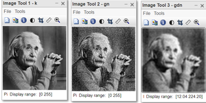
Figure: Gaussian noise

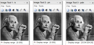
Figure: Poisson noise

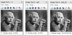
Figure: Salt and pepper noise

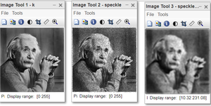
Figure: Speckle noise

Mean filter does not remove any particular noise effectively. 

Code Explanation:

• k=imread(“einstein_colored); This line reads the image.
• k=rgb2gray(k); this line converts into grayscale.
• gaussian_noise = imnoise(k, ‘gaussian’, 0, 0.01); this line creates the image corrupted with gaussian noise.
• gaussian_denoised=conv2(gaussian_noise, h, ‘same’); this line performs the convolution between gaussian_noisy image and mean filter.
• poisson_noise = imnoise(k, ‘poisson’); this line creates the image corrupted with poisson noise.
• poisson_denoised=conv2(poisson_noise, h, ‘same’); this line performs the convolution between poisson_noise image and mean filter.
• salt_noise = imnoise(k, ‘salt & pepper’, 0.05); this line creates the image corrupted with salt and pepper noise with 5 % of total pixels.
• salt_denoised=conv2(salt_noise, h, ‘same’); this line performs the convolution between salt_noise image and mean filter.
• speckle_noise = imnoise(k, ‘speckle’, 0.05); this line corrupts the image with speckle noise of 0.05 variance.
• speckle_denoised=conv2(speckle_noise, h, ‘same’); this line performs the convolution between speckle_noise image and mean filter.
• imtool(k, []); this line displays the original image.
• imtool(noised_image, []); this line displays the noisy_image.
• imtool(denoised_image, []); this line displays the denoised image.

Median Filter

A Median filter is a non-linear filter. It sorts the pixels covered by the window and sorts them in ascending order then returns the median of them.

For Median filter in the 2D image. We use medfit(). It takes 2 parameters. First is the noisy image, second is the window size used. By default window size is [3 3].

Syntax:

medfilt2( noisy_image, window_size);

To display the 2 images side by side together we use imshowpair().imshowpair( ) is an overloaded function, it has many signatures in Matlab. The montage keyword says that 2 images have to be displayed side by side. 

Syntax:

imshowpair(img1, img2, ‘montage’); 

Example:

Matlab

% MATLaB code for Median filter
% read the image.
k=imread("einstein_colored.png");

% Convert into grayscale image.
k=rgb2gray(k);

% Create the image corrupted with gaussian noise.
gaussian_noise=imnoise(k,'gaussian',0,0.01);

% Create the image corrupted with poisson noise.
poisson_noise=imnoise(k,'poisson');

% Create the image corrupted with salt
% & pepper noise.
salt_noise=imnoise(k,'salt & pepper', 0.05);

% Create the image corrupted
% with speckle noise.
speckle_noise=imnoise(k,'speckle', 0.05);

% Get the denoised image from noised
% image of: gaussian_noise
gaussian_denoised=medfilt2(gaussian_noise, [5 5]);

% Get the denoised image from
% noised image of:poisson_noise
poisson_denoised=medfilt2(poisson_noise, [5 5]);

% Get the denoised image from noised
% image of: salt_noise
salt_denoised=medfilt2(salt_noise, [5 5]);

% Get the denoised image from noised
% image of: speckle_noise
speckle_denoised=medfilt2(speckle_noise, [5 5]);

 % Display the noised and denoised image
 % side by side for Gaussian noise.
imshowpair(gaussian_noise, gaussian_denoised, 'montage');

 % Display the noised and denoised image
 %side by side for poisson_noise.
imshowpair(poisson_noise, poisson_denoised, 'montage');

% Display the noised and denoised
% image side by side for salt_noise.
imshowpair(salt_noise, salt_denoised, 'montage');

% Display the noised and denoised image
% side by side for speckle_noise.
imshowpair(speckle_noise, speckle_denoised, 'montage');

Output: 

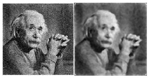
Figure: Gaussian noise

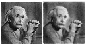
Figure:  Poisson noise

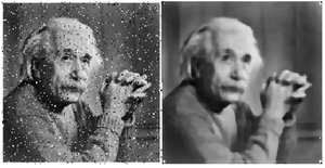
Figure: Salt and pepper noise

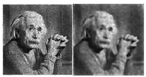
Figure: Speckle noise

The median filter removes the salt and pepper noise completely but introduces blurriness to the image. It does not perform well with other noises.

 Gaussian Filter

Syntax:

 B = imgaussfilt(A, sigma); // To obtain the filtered image using gaussian filter:

// imgaussfilt() is the built-in function in Matlab, which takes 2 parameters.

To display the noisy and denoised image side by side in single frame: imshowpair(P{noisy, denoised}); title(noisy vs denoised’);

Example:

Matlab

% MATLAB code using Gaussian Filter
% read the image.
k=imread("einstein_colored.jpg");

% convert to grayscale.
k=rgb2gray(k);

% create the image corrupted with gaussian noise
gaussian_noise=imnoise(k,'gaussian',0,0.01);

% create the image corrupted with poisson noise
poisson_noise=imnoise(k,'poisson');

% create the image corrupted with salt & pepper noise
salt_noise=imnoise(k,'salt & pepper', 0.05);

% create the image corrupted with speckle noise
speckle_noise=imnoise(k,'speckle', 0.05);

% get the denoised image from gaussian_noise image.
gaussian_denoised=imgaussfilt(gaussian_noise,1);

% get the denoised image from poisson_noise image.
poisson_denoised=imgaussfilt(poisson_noise, 1);

% get the denoised image from salt_noise image.
salt_denoised=imgaussfilt(salt_noise, 1);

% get the denoised image from speckle_noise image.
speckle_denoised=imgaussfilt(speckle_noise, 1);

% display noised and denoised images side by side.
montage({gaussian_noise,gaussian_denoised });
title('Gaussian noise and denoised image using gaussian filter');

% display noised and denoised images side by side.
montage({poisson_noise,poisson_denoised});
title('poisson noise img vs poisson denoised img');

% display noised and denoised images side by side.
montage({salt_noise,salt_denoised});
title('salt&pepper noise img vs denoised img');

% display noised and denoised images side by side.
montage({speckle_noise,speckle_denoised});
title('speckle noise img vs speckle denoised img');

Output:

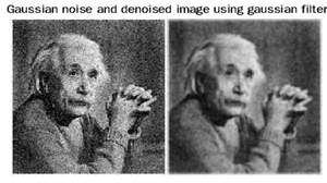
Figure: Gaussian noise

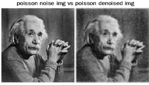
Figure: Poisson noise

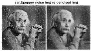
Figure: Salt and pepper noise

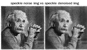
Figure: Speckle noise

Gaussian filter relatively works better with gaussian and poison noise. 

 Wiener Filter

• It is an adaptive low pass filtering technique.
• It filters the image pixel-wise.
• It is a type of linear filter.

Syntax:

J = wiener2(I,[m n],noise)

I = grayscale input image
[m n] = neighbouring window size

The wiener2 function applies a Wiener filter to an image adaptively. The Wiener filter sticks itself to the variance of the local image. Wiener2 performs little smoothing, wherever the variance is large. Wiener2 performs more smoothing, wherever the variance is small.

Syntax:

 k=imread(“einstein_colored); // To read the image:

 denoised=wiener2(noisy_image, [5 5]);

//To get the filtered image using Wiener filter

 imshowpair(P{noisy, denoised}); title(noisy vs denoised’);

//To display the noisy and denoised image side by side in single frame

here, weiner2( ) is an inbuilt function, it takes 2 parameters here. 1. Noisy image to be filtered2. Size of the neighboring window.

Example:

Matlab

% MATLAB code for Wiener2 filter
k=imread("einstein_colored.png");
k=rgb2gray(k);

% different noise with their parameters
gaussian_noise=imnoise(k,'gaussian',0,0.025);
poisson_noise=imnoise(k,'poisson');
salt_noise=imnoise(k,'salt & pepper', 0.05);
speckle_noise=imnoise(k,'speckle', 0.05);

% wiener filter with different noise
gaussian_denoised=wiener2(gaussian_noise, [5 5]);
poisson_denoised=wiener2(gaussian_noise, [5 5]);
salt_denoised=wiener2(salt_noise, [5 5]);
speckle_denoised=wiener2(speckle_noise, [5 5]);

imshowpair(gaussian_noise, gaussian_denoised, 'montage');
imshowpair(poisson_noise, poisson_denoised, 'montage');
imshowpair(salt_noise, salt_denoised, 'montage');
imshowpair(speckle_noise, speckle_denoised, 'montage');

Output:

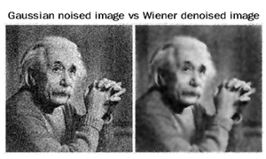
 Figure: Gaussian noise

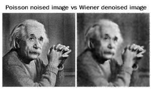
Figure: Poisson noise

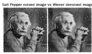
Figure: Salt and pepper noise

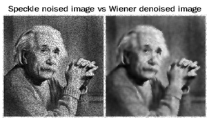
Figure: Speckle noise

Code Explanation:

• k=imread(“einstein_colored); This line reads the image.
• k=rgb2gray(k); this line converts into grayscale.
• gaussian_noise = imnoise(k, ‘gaussian’, 0, 0.01); this line creates the image corrupted with gaussian noise.
• poisson_noise = imnoise(k, ‘poisson’); this line creates the image corrupted with poisson noise.
• salt_noise = imnoise(k, ‘salt & pepper’, 0.05); this line creates the image corrupted with salt and pepper noise with 5 % of total pixels.
• speckle_noise = imnoise(k, ‘speckle’, 0.05); this line corrupts the image with speckle noise of 0.05 variance.
• gaussian_denoised=wiener2(gaussian_noise, [5 5]); this line applies the filter on gaussian noised image using window size [5 5]
• poisson_denoised=wiener2(gaussian_noise, [5 5]); this line applies the filter on poisson noised image using window size [5 5]
• salt_denoised=wiener2(salt_noise, [5 5]); this line applies the filter on gaussian salt and pepper image using window size [5 5]
• speckle_denoised=wiener2(speckle_noise, [5 5]); this line applies the filter on speckle noised image using window size [5 5]
• imshowpair(gaussian_noise, gaussian_denoised, ‘montage’); this line displays the gaussian noised image and denoised image side by side in the same frame.
• imshowpair(poisson_noise, poisson_denoised, ‘montage’); this line displays the poisson noised image and denoised image side by side in same frame.
• imshowpair(salt_noise, salt_denoised, ‘montage’); this line displays the salt and pepper noised image and denoised image side by side in same frame.
• imshowpair(speckle_noise, speckle_denoised, ‘montage’); this line displays the speckle noised image and denoised image side by side in same frame.

The adaptive approach often produces satisfactory results than linear filtering. The property of an adaptive filter is that it is more selective than a comparable linear filter because it preserves the edges and other high-frequency parts of an image.  There is one drawback of this, Wiener2 does require more computation time than another linear filtering.

When the noise is constant-power additive noise, such as Gaussian white noise; wiener2 gives the best results.