VLOOKUP On Multiple Criteria Columns Using Helper Method & CHOOSE Function

In this article, we will see how we can combine multiple values, and use them as lookup criteria for searching specific value(s) in the excel dataset. For this purpose, we will use the VLOOKUP formula, the most basic formula to perform a lookup for value(s) on excel. We will see a modified form of VLOOKUP to perform a lookup using multiple values.

First, let us see a general formula:

Formula:

=VLOOKUP(v1&v2,dataset_part,column,0)

Here,

• Here v1 and v2 signify those two cells, which will be used for lookup in combination.
• The Dataset_part signify the starting cell value and the ending cell value, upon which lookup is to be performed. This can consist of the whole dataset as well.
• The column signifies from which column the value has to be picked up.
• Here  0 signifies the approximation of lookup in vlookup. It can be set to 1 to enable approximation.

Now, let us see in brief, or a summary, how VLOOKUP will work in the Multiple Criteria Column. Here, we have 2 ways of modifying VLOOKUP to make it capable of doing a lookup on multiple criteria, they are:

1. Helper Column.
2. CHOOSE function.

Helper column will be a sort of redundant work, as we have to provide merged values of those columns on which VLOOKUP is doing the lookup, or we can use concatenation to concat the columns values. It should be kept in mind that the helper column should be the first column of our data. The CHOOSE function is usually preferred over creating a helper column in smaller datasets.

Now, let us see an example in both ways.

Using Helper Column:

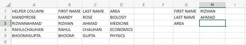
Now, let’s suppose we have this dataset with us. On the left side, the main dataset is written, and on the right side, a record has to be taken out from the main database. Now, you can either use CONCATENATE function, or you can manually write the merged values of your criteria columns in the helper column. Here, we want to know the area of study of RIZWAN AHMAD. But, we don’t know any other method than VLOOKUP to perform this. So, we will use VLOOKUP to achieve this. First, let us see the formula and understand it argument by argument.

=VLOOKUP(H1&H2,A2:D5,4,0)

The output of this will be:

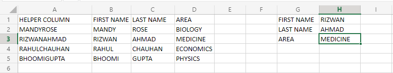
Now, we achieved the correct result, but how? Let’s look at it.

• H1&H2: The name is divided into 2 cells, which have been taken from criteria cells.
• A2:D5: The data is taken from this range.
• 4: This is the column number from which data will be retrieved,i.e from the AREA column.
• 0: This signifies that the approximation of lookup is turned off.

Here, the thing to keep in mind is that the helper column should always be created on the first column of the dataset.

Now, as discussed the helper column is not very much suited for smaller datasets. So, we will use CHOOSE function along with VLOOKUP to achieve the multiple criteria lookup.

Using CHOOSE Function:

Now, let’s suppose the given dataset is big, and we want to know the area of study of RIZWAN AHMAD, so for this, we will use CHOOSE function, which will help us create a 2D array, in which the search criteria values and other arguments will be stored and used.

Considering this dataset, the formula will be:

=VLOOKUP(H1&&H2,CHOOSE({1,2},B2:B5&&C2:C5,D2:D5),2,0)

Inserting this formula in H3, we will obtain the same output as obtained above. Now, how did this formula worked? Let’s look at argument by argument.

• H1&&H2: This will be the required value of searching. As we did not use the helper column, so we have to use the concatenated result. So, we used “&” to join or concatenate the name.
• {1,2}: This will create a 2D array, which will store the concatenated names, and the column of AREA, from which value will be fetched.
• B2:B5&&C2:C5: This will concatenate the two name columns and will store them in the first column of the 2D array created by the CHOOSE function.
• D2:D5: This will put the values of the AREA column in the second column of the 2D array created by CHOOSE function.
• 2: This number signifies which column of the 2D array has to be used to fetch the value, so in our case, it is the 2nd column(AREA).
• 0: This signifies that the approximation of lookup is turned off.

Note: If you want some separation between the concatenation, you can use any symbol, a blank space inside the “”(double quotes). Note that it should be placed in between && values, which are used for merging. So, for example, when merging H1 AND H2, but with some separation of blank space, we can write it as–>H1&” “&H2.

For large datasets, the helper column is preferred over CHOOSE function for doing multiple criteria lookup with VLOOKUP.