Visualizing training with TensorBoard
Last Updated :
05 Jul, 2021
In machine learning, to improve something you often need to be able to measure it. TensorBoard is a tool for providing the measurements and visualizations needed during the machine learning workflow. It enables tracking experiment metrics like loss and accuracy, visualizing the model graph, projecting NLP embeddings to a lower-dimensional space, and much more.
TensorBoard provides the following functionalities:
- Visualizing different metrics such as loss, accuracy with the help of different plots, and histograms.
- Visualize model layers and operations with the help of graphs.
- Provide histograms for weights and biases involved in training.
- Displaying training data (image, audio, and text data).
TensorBoard has the following tabs:
- Scalars: This tab is used to visualize the scalar metrics such as loss and accuracy.
- Graph: Visualize the computational graph of your models, such as the neural network model in the form layers and operations.
- Distributions: Visualize the training progression over time such as weight/bias changes.
- Histogram: Visualize the above distribution in the form of 3D-histograms.
- Projectors: This tab is used to visualize the word embedding for Natural Language Processing.
- Images: This tab is used to visualize the contents of training/test images data.
- Audio: This tab is used to visualize the audio data for application such as audio processing
- Text: This tab is used to visualize the audio data.
Implementation :
- Load TensorBoard extension:
Code:
python3
!pip install -q tf-nightly-2.0-preview
import tensorflow as tf
import datetime, os
logs_base_dir = "./logs"
os.makedirs(logs_base_dir, exist_ok=True)
%tensorboard --logdir {logs_base_dir}
|
Code:
python3
import numpy as np
import matplotlib.pyplot as plt
import io
!rm -rf ./logs/
cifar_10 = tf.keras.datasets.cifar10
(x_train, y_train), (x_test,y_test) = cifar_10.load_data()
class_names =["airplane","automobile","bird","cat","deer",
"dog","frog","horse", "ship","truck"]
x_train = x_train.astype('float32')
x_test = x_test.astype('float32')
x_train = x_train/255.0
x_test = x_test/255.0
y_train = tf.keras.utils.to_categorical(y_train)
y_test = tf.keras.utils.to_categorical(y_test)
logdir = "logs/train_data/" + datetime.now().strftime("%Y%m%d-%H%M%S")
file_writer = tf.summary.create_file_writer(logdir)
with file_writer.as_default():
images = np.reshape(x_train[0:25], (-1, 32, 32, 3))
tf.summary.image("Display training data", images, max_outputs=25, step=0)
%tensorboard --logdir logs/train_data
|
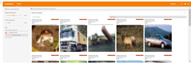
Training Images
- Plot Images Data Using Matplotlib: We can see that the above training images are not clear. That’s because the above training images are of size (32, 32, 3) which is of very low resolution. Let’s plot some images in matplotlib.
Code:
python3
!rm -rf logs/plots
logdir = "logs/plots/" + datetime.now().strftime("%Y%m%d-%H%M%S")
file_writer = tf.summary.create_file_writer(logdir)
def plot_to_image(figure):
buf = io.BytesIO()
plt.savefig(buf, format='png')
plt.close(figure)
buf.seek(0)
image = tf.image.decode_png(buf.getvalue(), channels=4)
print(image.shape)
image = tf.expand_dims(image, 0)
return image
def image_grid():
figure = plt.figure(figsize=(10,10))
for i in range(25):
plt.subplot(5, 5, i + 1, title = class_names[np.int(np.where(y_train[i] ==1)[0])])
plt.xticks([])
plt.yticks([])
plt.grid(False)
plt.imshow(x_train[i])
return figure
figure = image_grid()
with file_writer.as_default():
tf.summary.image("Training data", plot_to_image(figure), step=0)
%tensorboard --logdir logs/plots
|
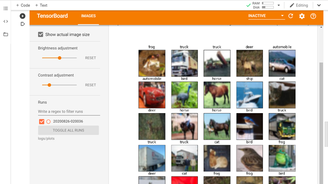
Training Images using matplotlib
- Display Training Results Metrics: In this section, we will be plotting results metrics on TensorBoard. We will be using scalars and images tabs to display our results. For that, we will define a Convolutional Neural Network model and train it on CIFAR 10 dataset for 20 epoch.
Code:
python3
model = tf.keras.models.Sequential([
tf.keras.layers.Conv2D(32, (3, 3), activation='relu', padding='same', input_shape=(32, 32, 3)),
tf.keras.layers.Conv2D(32, (3, 3), activation='relu', padding='same'),
tf.keras.layers.MaxPooling2D((2, 2)),
tf.keras.layers.Dropout(0.2),
tf.keras.layers.Conv2D(64, (3, 3), activation='relu', padding='same'),
tf.keras.layers.Conv2D(64, (3, 3), activation='relu', padding='same'),
tf.keras.layers.MaxPooling2D((2, 2)),
tf.keras.layers.Dropout(0.2),
tf.keras.layers.Flatten(),
tf.keras.layers.Dense(64, activation='relu'),
tf.keras.layers.Dense(10, activation='softmax')
])
model.compile(
optimizer=tf.keras.optimizers.SGD(learning_rate= 0.01 , momentum=0.1),
loss='categorical_crossentropy',
metrics=['accuracy']
)
model.summary()
|
Model: "sequential"
_________________________________________________________________
Layer (type)                 Output Shape              Param #
=================================================================
conv2d (Conv2D)              (None, 32, 32, 32)        896
_________________________________________________________________
conv2d_1 (Conv2D)            (None, 32, 32, 32)        9248
_________________________________________________________________
max_pooling2d (MaxPooling2D) (None, 16, 16, 32)        0
_________________________________________________________________
dropout (Dropout)            (None, 16, 16, 32)        0
_________________________________________________________________
conv2d_2 (Conv2D)            (None, 16, 16, 64)        18496
_________________________________________________________________
conv2d_3 (Conv2D)            (None, 16, 16, 64)        36928
_________________________________________________________________
max_pooling2d_1 (MaxPooling2 (None, 8, 8, 64)          0
_________________________________________________________________
dropout_1 (Dropout)          (None, 8, 8, 64)          0
_________________________________________________________________
flatten (Flatten)            (None, 4096)              0
_________________________________________________________________
dense (Dense)                (None, 64)                262208
_________________________________________________________________
dense_1 (Dense)              (None, 10)                650
=================================================================
Total params: 328,426
Trainable params: 328,426
Non-trainable params: 0
_________________________________________________________________
- Now, we define the function to plot the confusion matrix using test data
Code:
python3
def plot_confusion_matrix(cm, class_names):
figure = plt.figure(figsize=(8, 8))
plt.imshow(cm, interpolation='nearest', cmap=plt.cm.Blues)
plt.title("Confusion matrix")
plt.colorbar()
tick_marks = np.arange(len(class_names))
plt.xticks(tick_marks, class_names, rotation=45)
plt.yticks(tick_marks, class_names)
cm = np.around(cm.astype('float') / cm.sum(axis=1)[:, np.newaxis], decimals=2)
threshold = cm.max() / 2.
for i, j in itertools.product(range(cm.shape[0]), range(cm.shape[1])):
color = "white" if cm[i, j] > threshold else "black"
plt.text(j, i, cm[i, j], horizontalalignment="center", color=color)
plt.tight_layout()
plt.ylabel('True label')
plt.xlabel('Predicted label')
return figure
|
- Now, we define the TensorBoard callback to display the confusion matrix of the model predictions over test data.
Code:
python3
logdir = "logs/image/" + datetime.now().strftime("%Y%m%d-%H%M%S")
tensorboard_callback = tf.keras.callbacks.TensorBoard(log_dir=logdir)
file_writer_cm = tf.summary.create_file_writer(logdir + '/cm')
|
- Now, we define the function to log the confusion matrix into the Tensorboard.
Code:
python3
from sklearn.metrics import confusion_matrix
import itertools
def log_confusion_matrix(epoch, logs):
test_pred_raw = model.predict(x_test)
test_pred = np.argmax(test_pred_raw, axis=1)
y_test_cls = np.argmax(y_test, axis=1)
cm = confusion_matrix(y_test_cls, test_pred)
figure = plot_confusion_matrix(cm, class_names=class_names)
cm_image = plot_to_image(figure)
with file_writer_cm.as_default():
tf.summary.image("Confusion Matrix", cm_image, step=epoch)
cm_callback = tf.keras.callbacks.LambdaCallback(on_epoch_end=log_confusion_matrix)
|
Code:
python3
%tensorboard --logdir logs/image
model.fit(
x_train,
y_train,
epochs=20,
callbacks=[tensorboard_callback, cm_callback],
validation_data=(x_test, y_test)
)
|
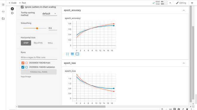
Loss & Accuracy Graph (Scalar Tab)
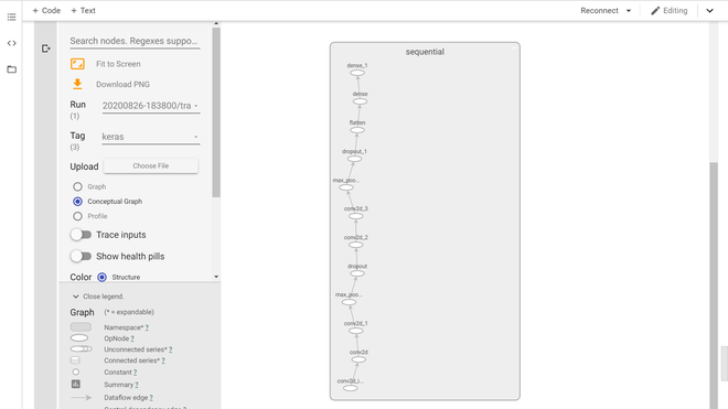
Keras Model Graph (Graph Tab)
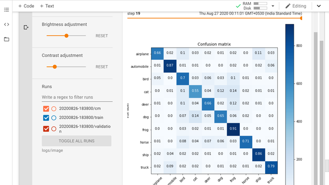
Confusion Matrix (Images Tab)
References:
Like Article
Suggest improvement
Share your thoughts in the comments
Please Login to comment...