Visualization of convents in Pytorch – Python

Convolutional Neural Networks (ConvNets or CNNs) are a category of Neural Networks that have proven very effective in areas such as image recognition and classification. Understanding the behavior of ConvNets can be a complex task, especially when working with large image datasets. To help with this, we can visualize the activations of individual neurons in ConvNets, which can provide us with insights into the features that the model is learning. In this article, we will explore how to visualize ConvNets using PyTorch, a popular deep-learning framework.

ConvNets: Convolutional Neural Networks are a type of neural network that is designed to work with image data. ConvNets are composed of several layers, including convolutional layers and pooling layers, which extract and reduce features from the input image.

Example 1 :

Step 1:

Install the necessary libraries

sudo apt install graphviz   # [Ubuntu]
winget install graphviz     # [Windows]
sudo port install graphviz  # [Mac]

pip install torchviz

Step 2:

Import the necessary libraries, including PyTorch, Numpy, and Matplotlib.

Python3

import torch
import torchvision
import torchvision.transforms as transforms
import torch.nn as nn
import torch.nn.functional as F
from PIL import Image
from torch.autograd import Variable
import torch.optim as optim
import matplotlib.pyplot as plt
import numpy as np
from torchviz import make_dot

Step 3:

Define the simple Convolution Neural Network model :

Python3

class convents(nn.Module):
    def __init__(self):
        super().__init__()
        self.conv1 = nn.Conv2d(3, 32, kernel_size=4, padding=1)
        self.conv2 = nn.Conv2d(32, 64, kernel_size=3, padding=1)
        self.pool = nn.MaxPool2d(2, 2)
        self.dropout1 = nn.Dropout2d(0.25)
        self.dropout2 = nn.Dropout2d(0.5)
        self.fc1 = nn.Linear(64 * 7 * 7, 128)
        self.fc2 = nn.Linear(128, 10)

    def forward(self, x):
        x = self.pool(F.relu(self.conv1(x)))
        x = self.dropout1(x)
        x = self.pool(F.relu(self.conv2(x)))
        x = self.dropout2(x)
        x = x.view(-1, 64 * 7 * 7)
        x = F.relu(self.fc1(x))
        x = self.fc2(x)
        return x

net = convents()

# Loss functions and optimizer
criterion = nn.CrossEntropyLoss()
optimizer = optim.SGD(net.parameters(), lr=0.001, momentum=0.9)

net

Output:

convents(
  (conv1): Conv2d(3, 32, kernel_size=(4, 4), stride=(1, 1), padding=(1, 1))
  (conv2): Conv2d(32, 64, kernel_size=(3, 3), stride=(1, 1), padding=(1, 1))
  (pool): MaxPool2d(kernel_size=2, stride=2, padding=0, dilation=1, ceil_mode=False)
  (dropout1): Dropout2d(p=0.25, inplace=False)
  (dropout2): Dropout2d(p=0.5, inplace=False)
  (fc1): Linear(in_features=3136, out_features=128, bias=True)
  (fc2): Linear(in_features=128, out_features=10, bias=True)
)

In the first conv1, the input will be 3 channels and the output will be 32 convolved images

Step 4:

Load the image

Python3

img = Image.open("Ganesh.jpg")
img

Output:

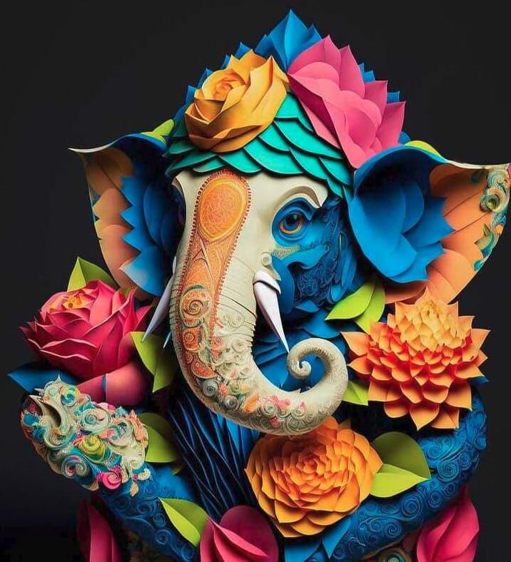
Input Image

Step 5:

Transform the image to Pytorch Tensor

Python3

# transform the image to pytorch tensor
transform = transforms.Compose([
    transforms.ToTensor(),
])


img = transform(img)
img.shape

Output:

torch.Size([3, 788, 716])

Step 6:

Get the first convolutional layer from our created model, and apply it to the image.

Python3

# Get activations of the first convolutional layer
conv1 = net.conv1
print('First convolution Layer :',conv1)

# APPLY THE FIRST Convolutional layer to the image
y = conv1(img)
print('Output Shape :',y.shape)

Output:

First convolution Layer : Conv2d(3, 32, kernel_size=(4, 4), stride=(1, 1), padding=(1, 1))
Output Shape : torch.Size([32, 787, 715])

We can visualize the convolution by torchviz make_dot functions. To use this graphviz should be installed in the system

Python3

make_dot(y.mean(), params=dict(conv1.named_parameters()))

Output:

Conv1 Visualizations

Step 7:

Get the weights of the first convolutional layer of the model.

Python3

# Get weights of the first convolutional layer
weights = conv1.weight.detach().numpy()
weights.shape

Output:

(32, 3, 4, 4)

Step 8:

Plot the Gray Scale original, Convolved, and Convolution weight with matplotlib

Python3

plt.figure(figsize =(12,5))

# Plot the original grayscale image
plt.subplot(1,3,1)
plt.imshow(img[0],cmap = 'gray')
plt.title('Original')
plt.axis('off')
img = Variable(img.unsqueeze(0), requires_grad=True)


#Plot the convolved grayscale image

# Squeeze tensor to numpy image
img_conv1 = y.detach().numpy()
img_conv1 = np.squeeze(img_conv1)

plt.subplot(1,3,2)
plt.imshow(img_conv1[0], cmap = 'gray')
plt.axis('off')
plt.title('After convolutions')

# Plot the weights of the first convolutional layer

# Squeeze tensor to numpy image
weights = np.squeeze(weights)

plt.subplot(1,3,3)
plt.imshow(weights[0,0,:,:], cmap='gray')
plt.axis('off')
plt.title('First convolutions weights')
plt.show()

Output:

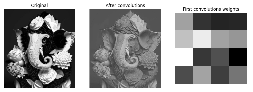
Original  & convolved Grayscale image with First convolutions weights

Example 2:

Let’s try a pre-trained model

• Import the necessary packages
• Load a pre-trained VGG16 model
• Load an image and transformed it
• Plot Original  & convolved Grayscale image with First convolutions weights
• visualize the convolution graph by torchviz 

Input Image:

Input Image

Code Implementations

Python3

# Import necessary libraries
import torch
import torchvision
import torchvision.transforms as transforms
import torchvision.models as models
import torch.nn as nn
import torch.nn.functional as F
from PIL import Image
from torch.autograd import Variable
import torch.optim as optim
import matplotlib.pyplot as plt
import numpy as np
from torchviz import make_dot

# Load a pre-trained VGG16 model
model = models.vgg16(pretrained=True)

# Transformations
transform = transforms.Compose([
    transforms.Resize(256),
    transforms.CenterCrop(224),
    transforms.ToTensor(),
    transforms.Normalize(mean=[0.485, 0.456, 0.406], std=[0.229, 0.224, 0.225])
])

# Load an example image and transformed it
img = transform(Image.open("GFG.img"))
#img = Variable(img.unsqueeze(0), requires_grad=True)

plt.figure(figsize =(12,5))
# Plot the original grayscale image
plt.subplot(1,3,1)
plt.imshow(img[0],cmap = 'gray')
plt.axis('off')
plt.title('Original')
img = Variable(img.unsqueeze(0), requires_grad=True)

# Get activations of the first convolutional layer
conv1 = model.features[0]

# APPLY THE FIRST Convolutional layer
y = conv1(img)
img_conv1 = y.detach().numpy()
img_conv1 = np.squeeze(img_conv1)

# Plot the convolved grayscale image
plt.subplot(1,3,2)
plt.imshow(img_conv1[0], cmap = 'gray')
plt.axis('off')
plt.title('After convolutions')


# Get weights of the first convolutional layer
weights = conv1.weight.detach().numpy()
weights = np.squeeze(weights)

# Plot the weights of the first convolutional layer
plt.subplot(1,3,3)
plt.imshow(weights[0,0,:,:], cmap='gray')
plt.axis('off')
plt.title('First convolutions weights')
plt.show()

make_dot(y.mean(), params=dict(conv1.named_parameters()))

Output:

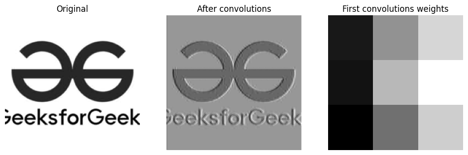
Original  & convolved Grayscale image with First convolutions weights

Conv1 Visualizations

Other ways to visualize ConvNets in PyTorch include plotting the weights of the convolutional layers, visualizing the filters in the convolutional layers, and plotting the feature maps produced by the activations of the convolutional layers. The choice of visualization will depend on the specific goals and questions you have about your ConvNet model.

In conclusion, visualizing the activations of ConvNets in PyTorch can provide valuable insights into the features that the model is learning and can help with understanding the behavior of the model.