Understanding High Leverage Point using Turicreate

High Leverage Point: A data point is considered to be a High Leverage Point if it has extreme predictor input value. An extreme input value simply means extremely low or extremely high value as compared to other data points in the entire Data set. The reason it is such an import concept in machine learning because it may highly influence your model fit on a particular data.

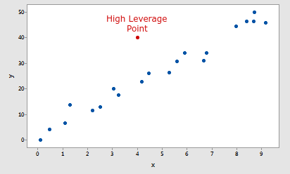
Example of a High Leverage Point

In this tutorial we are going to use turicreate to understand the concept of a high leverage point, so make sure you have turicreate installed in your system in order to follow along with the tutorial. For more info on Turicreate you can check this nice article on Turicreate.

So let’s understand this concept step by step.

Step 1: We will start by importing all the required libraries that we will need in this tutorial.

• Turicreate for fitting our regression model.
• Matplotlib for visualizing data.
• random for generating random numbers.

Python3

import turicreate
import matplotlib.pyplot as plt
import random

Step 2: Next, we will generate some data to fit our model and visualize the data using matplotlib.

Python3

#Creating data point for this tutorial
X = [random.randrange(1, 150) for i in range(200)]
Y = [random.randrange(200, 3000) for i in range(200)]

#Creating a separate point to demonstrate high leverage points
X.append(400)
Y.append(1000)

#Creating a SArray and SFRame
Xs = turicreate.SArray(X)
Ys = turicreate.SArray(Y)
data_points = turicreate.SFrame({"X" : Xs, "Y" : Ys})

#Plotting the Data
plt.scatter(Xs, Ys)
plt.xlabel("Input")
plt.ylabel("Output")
plt.show()

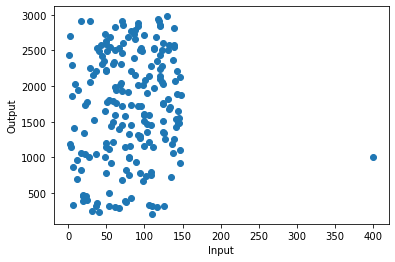
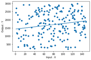
Output

As you can see in the image that there is a point in (400,1000) coordinate which is very far along the x-axis as compared to other data. That point is called High Leverage Point.

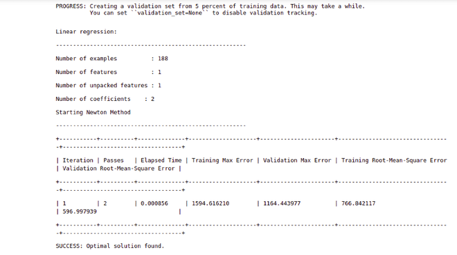
Step 3: Now, we will fit a regression model on our data.

Python3

#Fitting a linear Regression model with the given data
model = turicreate.linear_regression.create(data_points,
                                            target = "Y",
                                            features = ["X"])

#Plotting the fitted model
plt.scatter(data_points["X"], data_points["Y"])
plt.xlabel("Input : X")
plt.ylabel("Output : Y")
plt.plot(data_points["X"], model.predict(data_points))
plt.show()

Output

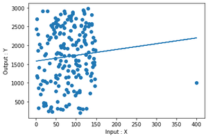
plot of the fit

Step 4 : Now again fit the regression model but this time we will remove the high leverage data point.

Python3

#Training the regression model with the data that do not
#contain high leverage point
model_nohlp = turicreate.linear_regression.create(
  data_points_with_no_high_leverage_points, target = "Y", features = ["X"])

#Plotting the fitted model having no high leverage point
plt.scatter(data_points_with_no_high_leverage_points["X"],
            data_points_with_no_high_leverage_points["Y"])
plt.xlabel("Input : X")
plt.ylabel("Output : Y")
plt.plot(data_points_with_no_high_leverage_points["X"],
         model_nohlp.predict(data_points_with_no_high_leverage_points))
plt.show()

Output

plot of the fit

Step 5: As of now you cannot determine the actual difference between the two models. So let’s visualize these two fits in the same picture to better understand the difference.

Python3

#Plotting both the fitted model in order to compare the results better
plt.scatter(data_points["X"], data_points["Y"], label = "Data Points")
plt.xlabel("Input : X")
plt.ylabel("Output : Y")

plt.plot(data_points["X"], model.predict(data_points),
         label = "Model with High leverage Point")
plt.plot(data_points_with_no_high_leverage_points["X"],
         model_nohlp.predict(data_points_with_no_high_leverage_points),
         label = "Model with no High Leverage point")

plt.legend()
plt.show()

Python3

#Plotting both the fitted model in order to compare the results better
plt.scatter(data_points["X"], data_points["Y"], label = "Data Points")
plt.xlabel("Input : X")
plt.ylabel("Output : Y")

plt.plot(data_points["X"], model.predict(data_points),
         label="Model with High leverage Point")

plt.plot(data_points_with_no_high_leverage_points["X"],
         model_nohlp.predict(data_points_with_no_high_leverage_points),
         label = "Model with no High Leverage point")

plt.legend()
plt.show()

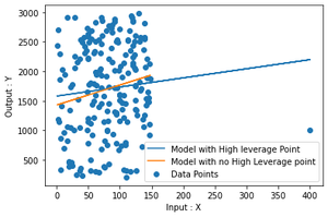
Output

As you can clearly see in the plot that there is a little difference between the two plot that arises just by removing a single point.

Step 6: Now we will calculate the actual difference between these two fits. For this, we will calculate the regression coefficients of both the model.

Python3

#Comparing the regression coefficients of both the models
print(f"""
Model with High Leverage Point
{model.coefficients}
-----------------------------------------------------------------------
-----------------------------------------------------------------------
Model without High Leverage Point
{model_nohlp.coefficients}
""")

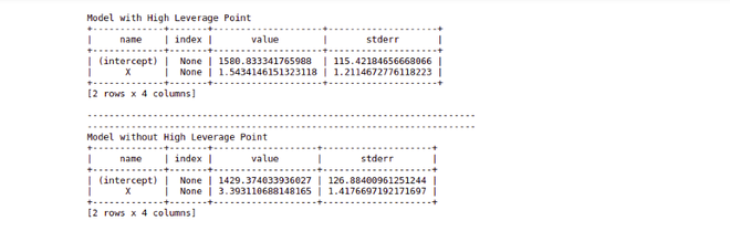
Output

As it is clearly visible from the picture that the difference between the coefficients of the two models is not that big, however in real-world projects where there is actual data and amount of data is really huge, it may highly influence the fit of the model but still, an analyst needs to find out whether a data point is actually high leverage or not without jumping to any conclusion. 

In this case, we are using simple linear regression to fit our data, so we can just simply visualize the data in a 2-D plot, but we don’t have that luxury in the case of multiple linear regression. In that situation, we have to rely on various measures to help us determine whether a data point is a high leverage point or not.