Understanding Activation Functions in Depth
Last Updated :
03 Jan, 2022
What is an Activation function ?
In artificial neural networks, the activation function of a node defines the output of that node or neuron for a given input or set of inputs. This output is then used as input for the next node and so on until a desired solution to the original problem is found.
It maps the resulting values into the desired range such as between 0 to 1
or -1 to 1 etc. It depends upon the choice of the activation function. For example, the use of the logistic activation function would map all inputs in the real number domain into the range of 0 to 1.
Example of a binary classification problem:
In a binary classification problem, we have an input x, say an image, and we have to classify it as having a correct object or not. If it is a correct object, we will assign it a 1, else 0. So here, we have only two outputs – either the image contains a valid object or it does not. This is an example of a binary classification problem.
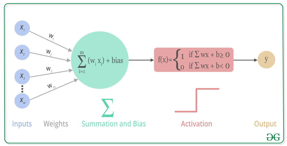
when we multiply each of them features with a weight (w1, w2, …, wm) and sum them all together,
node output = activation(weighted sum of inputs).
(1) 
`
Some Important terminology and mathematical concept –
-
Propagation is a procedure to repeatedly adjust the weights so as to minimize the difference between actual output and desired output.
-
Hidden Layers is which are neuron nodes stacked in between inputs and outputs, allowing neural networks to learn more complicated features (such as XOR logic).
-
Backpropagation is a procedure to repeatedly adjust the weights so as to minimize the difference between actual output and desired output.
It allows the information to go back from the cost backward through the network in order to compute the gradient. Therefore, loop over the nodes starting from the final node in reverse topological order to compute the derivative of the final node output. Doing so will help us know who is responsible for the most error and change the parameters appropriate in that direction.
-
Gradient Descent is used while training a machine learning model. It is an optimization algorithm, based on a convex function, that tweaks its parameters iteratively to minimize a given function to its local minimum. A gradient measures how much the output of a function changes if you change the inputs a little bit.
Note: If gradient descent is working properly, the cost function should decrease after every iteration.
Types of activation Functions:
The Activation Functions are basically two types:
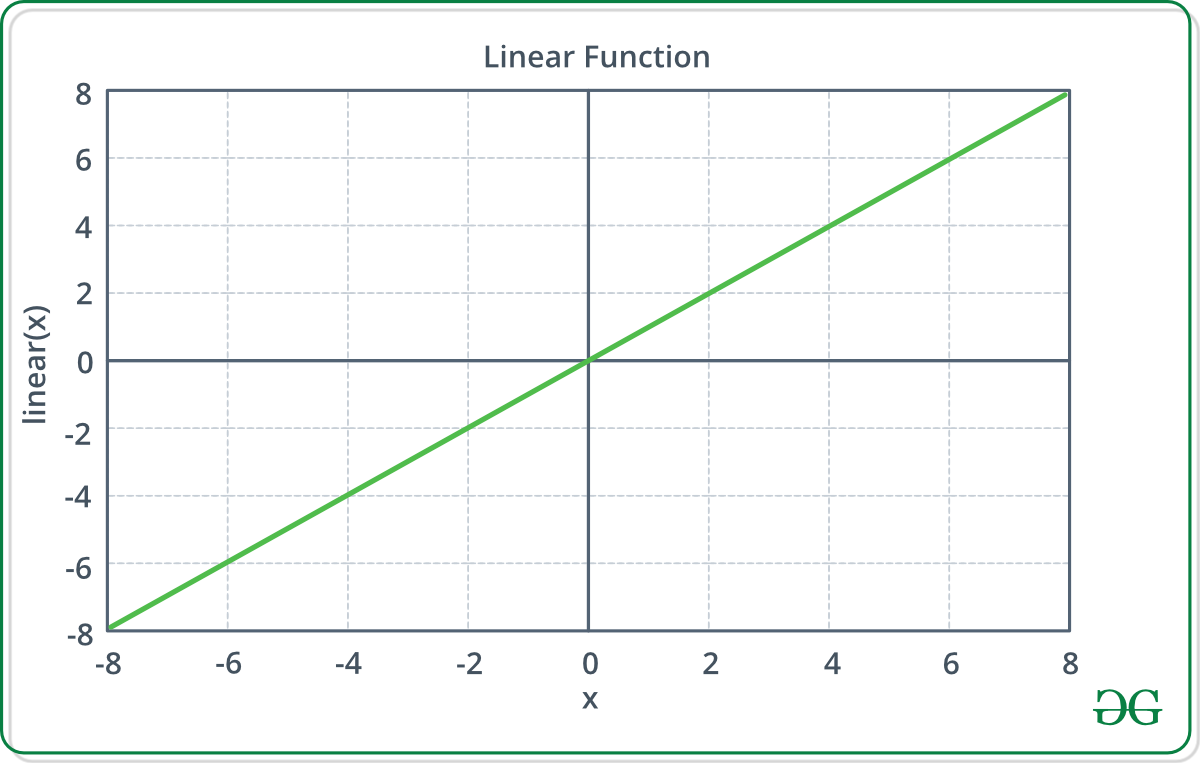
1. Linear Activation Function –
Equation : f(x) = x
Range : (-infinity to infinity)
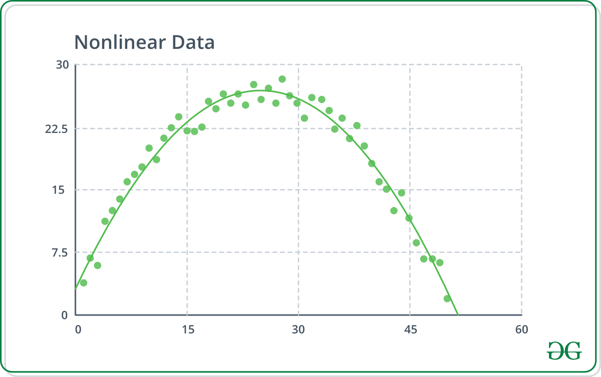
 2. Non-linear Activation Functions –
It makes it easy for the model to generalize with a variety of data and to differentiate between the output. By simulation, it is found that for larger networks ReLUs is much faster. It has been proven that ReLUs result in much faster training for large networks. Non-linear means that the output cannot be reproduced from a linear combination of the inputs.
The main terminologies needed to understand for nonlinear functions are:
1. Derivative: Change in y-axis w.r.t. change in x-axis. It is also known as slope.
2. Monotonic function: A function which is either entirely non-increasing or non-decreasing.
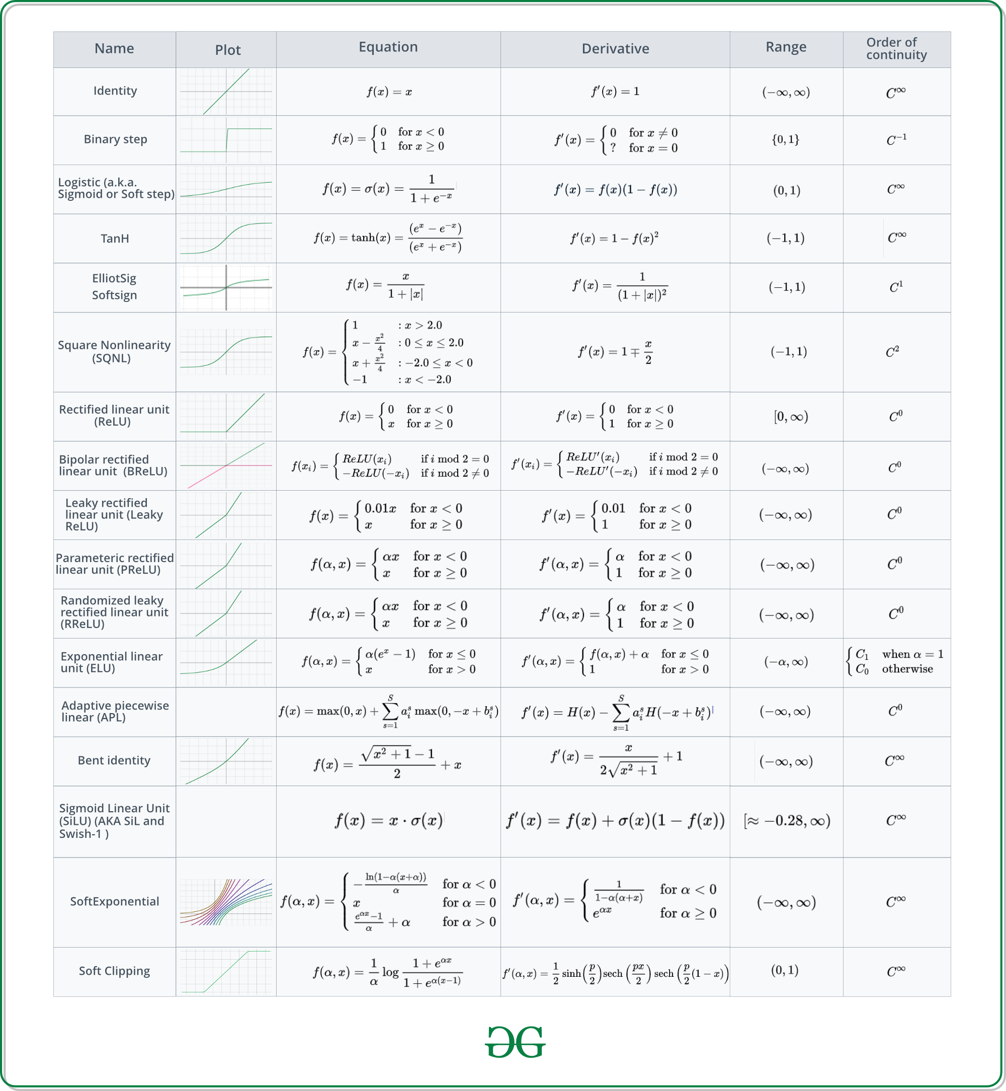
 The Nonlinear Activation Functions are mainly divided on the basis of their range or curves as follows:
 Let’s take a deeper insight in each Activations Functions-
1. Sigmoid:
Let’s take a deeper insight in each Activations Functions-
1. Sigmoid:
It is also called as a
Binary classifier or
Logistic Activation function because function always pick value either 0(False) or 1 (True).
The sigmoid function produces similar results to step function in that the output is between 0 and 1. The curve crosses 0.5 at z=0, which we can set up rules for the activation function, such as: If the sigmoid neuron’s output is larger than or equal to 0.5, it outputs 1; if the output is smaller than 0.5, it outputs 0.
The sigmoid function does not have a jerk on its curve. It is smooth and it has a very nice and simple derivative, which is differentiable everywhere on the curve.
Derivation of Sigmoid:
![Let's denote the sigmoid function as $\sigma(x)=\frac{1}{1+e^{x}}$. The derivative of the sigmoid is $\frac{d}{d x} \sigma(x)=\sigma(x)(1-\sigma(x))$. Here's a detailed derivation: $$ \begin{aligned} \frac{d}{d x} \sigma(x) &=\frac{d}{d x}\left[\frac{1}{1+e^{x}}\right] \\ &=\frac{d}{d x}\left(1+\mathrm{e}^{-x}\right)^{-1} \\ &=-\left(1+e^{-x}\right)^{-2}\left(-e^{-x}\right) \\ &=\frac{e^{-z}}{\left(1+e^{x}\right)^{2}} \\ &=\frac{1}{1+e^{-z}} \cdot \frac{e^{x}}{1+e^{-z}} \\ &=\frac{1}{1+e^{-}} \cdot \frac{\left(1+e^{-x}\right)-1}{1+e^{-x}} \\ &=\frac{1}{1+e^{-z}} \cdot\left(\frac{1+e^{-z}}{1+e^{-z}}-\frac{1}{1+e^{-z}}\right) \\ &=\frac{1}{1+e^{-z}} \cdot\left(1-\frac{1}{1+e^{-x}}\right) \\ &=\sigma(x) \cdot(1-\sigma(x)) \end{aligned} $$](https://www.geeksforgeeks.org/wp-content/ql-cache/quicklatex.com-a6104dd1ce42fa45a55fc7f3b12621fc_l3.png "Rendered by QuickLaTeX.com")
Sigmoids saturate and kill gradients. A very common property of the sigmoid is that when the neuron’s activation saturates at either 0 or 1, the gradient at these regions is almost zero. Recall that during backpropagation, this local gradient will be multiplied by the gradient of this gate’s output for the whole objective. Therefore, if the local gradient is very small, it will effectively “kill” the gradient and almost no signal will flow through the neuron to its weights and recursively to its data. Additionally, the extra penalty will be added initializing the weights of sigmoid neurons to prevent saturation. For example, if the initial weights are too large then most neurons would become saturated and the network will barely learn.
2. ReLU (Rectified Linear Unit):
It is the most widely used activation function. Since it is used in almost all the convolutional neural networks. ReLU is half rectified from the bottom. The function and it’s derivative both are monotonic.
f(x) = max(0, x)
The models that are close to linear are easy to optimize. Since ReLU shares a lot of the properties of linear functions, it tends to work well on most of the problems. The only issue is that the derivative is not defined at z = 0, which we can overcome by assigning the derivative to 0 at z = 0. However, this means that for z <= 0 the gradient is zero and again can’t learn.
3. Leaky ReLU:
Leaky ReLU is an improved version of the ReLU function. ReLU function, the gradient is 0 for x<0, which made the neurons die for activations in that region. Leaky ReLU is defined to address this problem. Instead of defining the Relu function as 0 for x less than 0, we define it as a small linear component of x.
Leaky ReLUs are one attempt to fix the Dying ReLU problem. Instead of the function being zero when x < 0, a leaky ReLU will instead have a small negative slope (of 0.01, or so). That is, the function computes:
(2) 
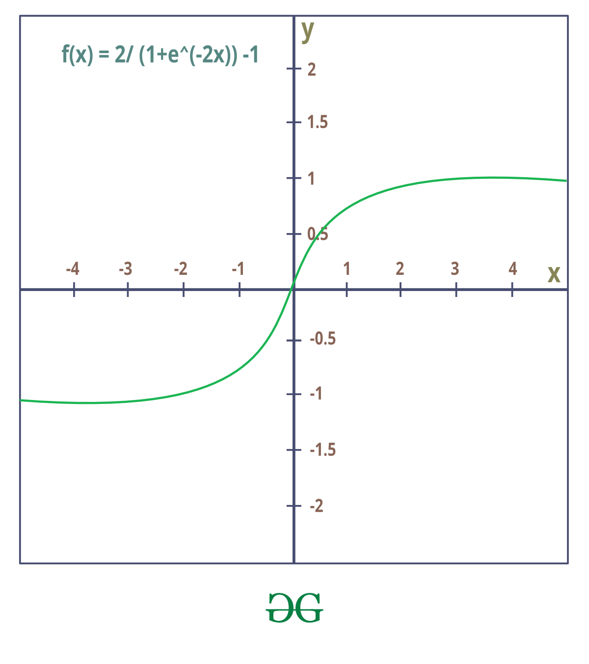
4. Tanh or hyperbolic tangent:
It squashes a real-valued number to the range [-1, 1] Like the Sigmoid, its activations saturate, but unlike the sigmoid neuron, its output is zero-centred. Therefore the tanh non-linearity is always preferred to the sigmoid nonlinearity. tanh neuron is simply a scaled sigmoid neuron.
Tanh is also like logistic sigmoid but better. The advantage is that the negative inputs will be mapped to strongly negative and the zero inputs will be mapped to near zero in the tanh graph.
The function is differentiable monotonic but its derivative is not monotonic. Both tanh and logistic Sigmoid activation functions are used in feed-forward nets.
It is actually just a scaled version of the sigmoid function.
tanh(x)=2 sigmoid(2x)-1
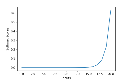
 5. Softmax :
The sigmoid function can be applied easily and ReLUs will not vanish the effect during your training process. However, when you want to deal with classification problems, they cannot help much. the sigmoid function can only handle two classes, which is not what we expect but we want something more. The softmax function squashes the outputs of each unit to be between 0 and 1, just like a sigmoid function. and it also divides each output such that the total sum of the outputs is equal to 1.
The output of the softmax function is equivalent to a categorical probability distribution, it tells you the probability that any of the classes are true.
where 0 is a vector of the inputs to the output layer (if you have 10 output units, then there are 10 elements in z). And again, j indexes the output units, so j = 1, 2, …, K.
Properties of Softmax Function –
1. The calculated probabilities will be in the range of 0 to 1.
2. The sum of all the probabilities is equals to 1.
Softmax Function Usage –
1. Used in multiple classification logistic regression model.
2. In building neural networks softmax functions used in different layer level and multilayer perceptrons.
Example:
(3) ![\begin{equation*} \left[\begin{array}{l} 1.2 \\ 0.9 \\ 0.4 \end{array}\right] \longrightarrow \operatorname{Softmax} \longrightarrow\left[\begin{array}{l} 0.46 \\ 0.34 \\ 0.20 \end{array}\right] \end{equation*}](https://www.geeksforgeeks.org/wp-content/ql-cache/quicklatex.com-b2fb3a8f84c1973c800df7e678702a01_l3.png "Rendered by QuickLaTeX.com")
Softmax function turns logits [1.2, 0.9, 0.4] into probabilities [0.46, 0.34, 0.20], and the probabilities sum to 1.
Like Article
Suggest improvement
Share your thoughts in the comments
Please Login to comment...