Types of Boltzmann Machines

Deep Learning models are broadly classified into supervised and unsupervised models. 

Supervised DL models:

• Artificial Neural Networks (ANNs)
• Recurrent Neural Networks (RNNs)
• Convolutional Neural Networks (CNNs)

Unsupervised DL models:

• Self Organizing Maps (SOMs)
• Boltzmann Machines
• Autoencoders

Let us learn what exactly Boltzmann machines are, how they work and also implement a recommender system which recommends whether the user likes a movie or not based on the previous movies watched.

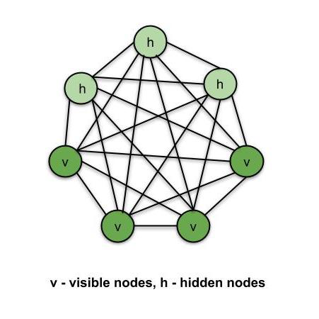
Boltzmann Machines is an unsupervised DL model in which every node is connected to every other node. That is, unlike the ANNs, CNNs, RNNs and SOMs, the Boltzmann Machines are undirected (or the connections are bidirectional). Boltzmann Machine is not a deterministic DL model but a stochastic or generative DL model. It is rather a representation of a certain system. There are two types of nodes in the Boltzmann Machine — Visible nodes — those nodes which we can and do measure, and the Hidden nodes – those nodes which we cannot or do not measure. Although the node types are different, the Boltzmann machine considers them as the same and everything works as one single system. The training data is fed into the Boltzmann Machine and the weights of the system are adjusted accordingly. Boltzmann machines help us understand abnormalities by learning about the working of the system in normal conditions.

Boltzmann Machine

Energy-Based Models:

Boltzmann Distribution is used in the sampling distribution of the Boltzmann Machine. The Boltzmann distribution is governed by the equation –

Pi = e(-∈i/kT)/ ∑e(-∈j/kT)          
Pi - probability of system being in state i
∈i - Energy of system in state i
T - Temperature of the system
k - Boltzmann constant
∑e(-∈j/kT) - Sum of values for all possible states of the system 

Boltzmann Distribution describes different states of the system and thus Boltzmann machines create different states of the machine using this distribution. From the above equation, as the energy of system increases, the probability for the system to be in state ‘i’ decreases. Thus, the system is the most stable in its lowest energy state (a gas is most stable when it spreads). Here, in Boltzmann machines, the energy of the system is defined in terms of the weights of synapses. Once the system is trained and the weights are set, the system always tries to find the lowest energy state for itself by adjusting the weights.

Types of Boltzmann Machines:

• Restricted Boltzmann Machines (RBMs)
• Deep Belief Networks (DBNs)
• Deep Boltzmann Machines (DBMs)

Restricted Boltzmann Machines (RBMs):

In a full Boltzmann machine, each node is connected to every other node and hence the connections grow exponentially. This is the reason we use RBMs. The restrictions in the node connections in RBMs are as follows –

• Hidden nodes cannot be connected to one another.
• Visible nodes connected to one another.

Energy function example for Restricted Boltzmann Machine –

E(v, h) = -∑ aivi - ∑ bjhj - ∑∑ viwi,jhj
a, v - biases in the system - constants
vi, hj - visible node, hidden node
P(v, h) = Probability of being in a certain state
P(v, h) = e(-E(v, h))/Z
Z - sum if values for all possible states

Suppose that we are using our RBM for building a recommender system that works on six (6) movies. RBM learns how to allocate the hidden nodes to certain features. By the process of Contrastive Divergence, we make the RBM close to our set of movies that is our case or scenario. RBM identifies which features are important by the training process. The training data is either 0 or 1 or missing data based on whether a user liked that movie (1), disliked that movie (0) or did not watch the movie (missing data). RBM automatically identifies important features. 

Contrastive Divergence:

RBM adjusts its weights by this method. Using some randomly assigned initial weights, RBM calculates the hidden nodes, which in turn use the same weights to reconstruct the input nodes. Each hidden node is constructed from all the visible nodes and each visible node is reconstructed from all the hidden node and hence, the input is different from the reconstructed input, though the weights are the same. The process continues until the reconstructed input matches the previous input. The process is said to be converged at this stage. This entire procedure is known as Gibbs Sampling. 

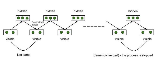
Gibb’s Sampling

The Gradient Formula gives the gradient of the log probability of the certain state of the system with respect to the weights of the system. It is given as follows –

d/dwij(log(P(v0))) = <vi0 * hj0> - <vi∞ * hj∞>
v - visible state, h- hidden state
<vi0 * hj0> - initial state of the system
<vi∞ * hj∞> - final state of the system
P(v0) - probability that the system is in state v0
wij - weights of the system

The above equations tell us – how the change in weights of the system will change the log probability of the system to be a particular state. The system tries to end up in the lowest possible energy state (most stable). Instead of continuing the adjusting of weights process until the current input matches the previous one, we can also consider the first few pauses only. It is sufficient to understand how to adjust our curve so as to get the lowest energy state. Therefore, we adjust the weights, redesign the system and energy curve such that we get the lowest energy for the current position. This is known as the Hinton’s shortcut.

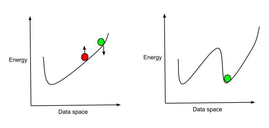
Hinton’s Shortcut

Working of RBM – Illustrative Example –

Consider – Mary watches four movies out of the six available movies and rates four of them. Say, she watched m₁, m₃, m₄ and m₅ and likes m₃, m₅ (rated 1) and dislikes the other two, that is m₁, m₄ (rated 0) whereas the other two movies – m2, m6 are unrated. Now, using our RBM, we will recommend one of these movies for her to watch next. Say – 

• m₃, m₅ are of ‘Drama’ genre.
• m₁, m₄ are of ‘Action’ genre.
• ‘Dicaprio’ played a role in m₅.
• m₃, m₅ have won ‘Oscar.’
• ‘Tarantino’ directed m₄.
• m₂ is of the ‘Action’ genre.
• m₆ is of both the genres ‘Action’ and ‘Drama’, ‘Dicaprio’ acted in it and it has won an ‘Oscar’.

We have the following observations –

• Mary likes m₃, m₅ and they are of genre ‘Drama,’ she probably likes ‘Drama’ movies.
• Mary dislikes m₁, m₄ and they are of action genre, she probably dislikes ‘Action’ movies.
• Mary likes m₃, m₅ and they have won an ‘Oscar’, she probably likes an ‘Oscar’ movie.
• Since ‘Dicaprio’ acted in m₅ and Mary likes it, she will probably like a movie in which ‘Dicaprio’ acted.
• Mary does not like m₄ which is directed by Tarantino, she probably dislikes any movie directed by ‘Tarantino’.

Therefore, based on the observations and the details of m₂, m₆; our RBM recommends m6 to Mary (‘Drama’, ‘Dicaprio’ and ‘Oscar’ matches both Mary’s interests and m₆). This is how an RBM works and hence is used in recommender systems.

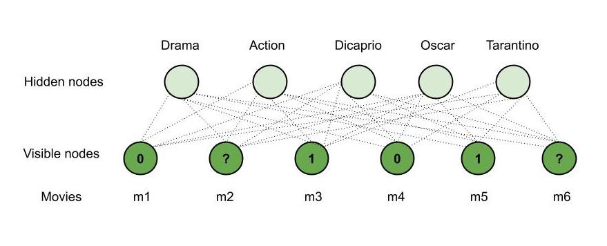
Working of RBM

Thus, RBMs are used to build Recommender Systems.

Deep Belief Networks (DBNs):

Suppose we stack several RBMs on top of each other so that the first RBM outputs are the input to the second RBM and so on. Such networks are known as Deep Belief Networks. The connections within each layer are undirected (since each layer is an RBM). Simultaneously, those in between the layers are directed (except the top two layers – the connection between the top two layers is undirected). There are two ways to train the DBNs-

1. Greedy Layer-wise Training Algorithm – The RBMs are trained layer by layer. Once the individual RBMs are trained (that is, the parameters – weights, biases are set), the direction is set up between the DBN layers.
2. Wake-Sleep Algorithm – The DBN is trained all the way up (connections going up – wake) and then down the network (connections going down — sleep).

Therefore, we stack the RBMs, train them, and once we have the parameters trained, we make sure that the connections between the layers only work downwards (except for the top two layers).

Deep Boltzmann Machines (DBMs):

DBMs are similar to DBNs except that apart from the connections within layers, the connections between the layers are also undirected (unlike DBN in which the connections between layers are directed). DBMs can extract more complex or sophisticated features and hence can be used for more complex tasks.