Two-Tailed Test of Population Mean with Unknown Variance in R

Conventionally, In a two-tail test, the null hypothesis states that the true population mean (μo) is equal to the hypothesized mean value (μ). We fail to reject the null hypothesis if the test statistic lies within the range of critical values at the chosen significance level. In this article let us discuss the probability percentage of type II error for a two-tail test of the population mean with unknown variance.

Type II error is an error that occurs if the hypothesis test based on a random sample fails to reject the null hypothesis even when the true population means μo is not equal to the hypothesized mean value μ.

Here the assumption is the population variance σ2  is unknown. Let s2 be the sample variance. For larger n (usually >30), the population of the following statistics of all possible samples of size n is approximately a Student t distribution with n – 1 degree of freedom (DOF).

The test statistic is defined as 

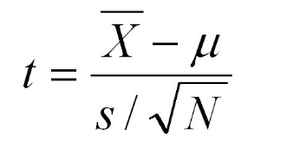
test statistic

The null hypothesis of the two-tailed test can be rejected if t ≤−tα∕2 or t ≥ tα∕2, where tα∕2 is the 100(1 − α) percentile of the Student t distribution with n − 1 degree of freedom. Here, alpha is the chosen significance level.

Let us try to understand the Two-Tailed Test of Population Mean with Unknown Variance by considering a case study.

Suppose the mean weight of boxers in Asia last year was 75.4 kg. In a sample of 35 boxers same time this year in the same region, the mean boxer’s weight is 74.6 kg. Assume the sample standard deviation is 2.5 kg. At the .05 significance level, can we reject the null hypothesis that the mean boxer’s weight does not differ from last year?

Example:

Let us compute the test statistic t,

R

xbar = 74.6 # sample mean
mu0 = 75.4 # hypothesized value
s = 2.5 # sample standard deviation
n = 35 # sample size
t = (xbar-mu0)/(s/sqrt(n))
t # test statistic

Output:

-1.8931455305919

Now let’s compute the critical values at .05 significance level.

R

alpha = .05
t.half.alpha = qt(1-alpha/2, df=n-1)
c(-t.half.alpha, t.half.alpha)

Output:

-2.03224450931772  2.03224450931772

The range of critical values (-2.03 – +2.03) suggests that the test statistic -1.89 lies very well within the range. Hence, at the .05 significance level, we do not reject the null hypothesis that the mean boxer’s weight does not differ from last year.