Two-Tailed Test of Population Mean with Known Variance in R

A statistical hypothesis test is a method of statistical inference used to decide whether the data at hand sufficiently support a particular hypothesis.

The conventional steps that are followed while formulating the hypothesis test, are listed as follows

• State null hypothesis (Ho) and alternate hypothesis (Ha)
• Collect a relevant sample of data to test the hypothesis.
• Choose significance level for the hypothesis test.
• Perform an appropriate statistical test.
• Based on test statistics and p-value decide whether to reject or fail to reject your null hypothesis.

Two-tailed test

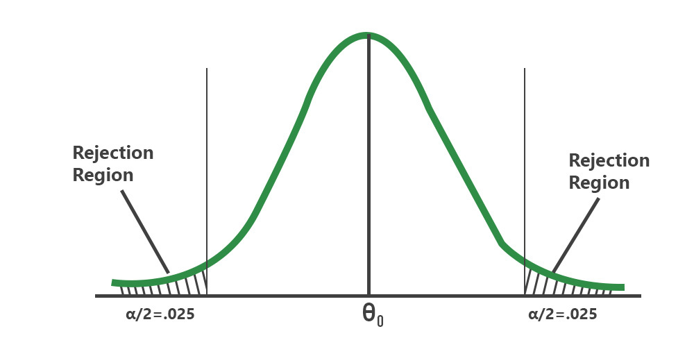
Conventionally, In a two-tailed test, the null hypothesis states that the true population mean (μo) is equal to the hypothesized mean value (μ). We fail to reject the null hypothesis if the test statistic is equal to the critical value at the chosen significance level. In this article let us discuss how to conduct a two-tail test of the population mean with known variance.

Here the assumption is the population variance σ2  is known. From Central Limit Theorem (CLT), the population. the sample means of all possible samples of a population approximately follow a normal distribution. Let us define the test statistic based on CLT as follows

If z <= −z_α/2  or z >=z_α/2, where z_α/2 is the 100(1 − α/2) percentile of the standard normal distribution, we will have to reject the null hypothesis.

Let us try to understand the type II error by considering a case study.

Suppose the mean weight of boxers in Asia last year was 75.4 kg. In a sample of 35 boxers same time this year in the same region, the mean boxer’s weight is 74.6 kg. Assume the population standard deviation is 2.5 kg. At the .05 significance level, can we reject the null hypothesis that the mean boxer’s weight does not differ from last year?

Example:

The null hypothesis is that μ = 75.4. Let us compute the test statistic.

R

# sample mean
sample_mean = 74.6

# hypothesized mean
m0 = 75.4

# population standard deviation
pop_std_dev = 2.5

# sample size
sample_size = 35
z = (sample_mean-m0)/(pop_std_dev/sqrt(sample_size))
z

Output:

-1.8931

R

# significance level
alpha = .05

# upper and lower bound
z.half.alpha = qnorm(1-alpha/2)
c(-z.half.alpha, z.half.alpha)

Output:

-1.96   1.96

The range of the critical values (-1.96 – +1.96) suggests that the test statistic -1.8931 lies well within the range. Hence, at the .05 significance level, we do not reject the null hypothesis that the mean boxer’s weight does not differ from last year.