Training of Recurrent Neural Networks (RNN) in TensorFlow

In this article, we shall train an RNN i.e., Recurrent Neural Networks(RNN) in TensorFlow. TensorFlow makes it effortless to build a Recurrent Neural Network without performing its mathematics calculations. Compare to other Deep Learning frameworks, TensorFlow is the easiest way to build and train a Recurrent Neural Network. 

Recurrent Neural Networks in TensorFlow

Recurrent Neural Network is different from Convolution Neural Network and Artificial Neural Network. A Neural Network is basically known to be trained to learn deep features to make accurate predictions. Whereas Recurrent Neural Network works in such a way that there is feedback between each node which stores information in the cell state. In simple words, Recurrent Neural Networks are the process of backpropagating through time. 

In the later part of the article, we all discuss why to use Bidirectional RNN Gated Architecture. To implement the training of Recurrent Neural Networks (RNN) in TensorFlow, let’s work on some real-time NLP projects. 

Importing Libraries and Dataset

Python libraries make it very easy for us to handle the data and perform typical and complex tasks with a single line of code.

• Pandas – This library helps to load the data frame in a 2D array format and has multiple functions to perform analysis tasks in one go.
• Numpy – Numpy arrays are very fast and can perform large computations in a very short time.
• Matplotlib/Seaborn – This library is used to draw visualizations.
• TensorFlow – Import TensorFlow and Keras API that comes installed with TensorFlow. Keras API helps in building a Neural Network in just a few lines of code.
• NLTK – Natural Language Processing Toolkit comes in very handy while handling raw textual data.
• Sklearn – This module contains multiple libraries having pre-implemented functions to perform tasks from data preprocessing to model development and evaluation.

Python3

import warnings
from tensorflow.keras.utils import pad_sequences
from tensorflow.keras.preprocessing.text import Tokenizer
from sklearn.model_selection import train_test_split
import tensorflow as tf
from tensorflow import keras
import pandas as pd
import matplotlib.pyplot as plt
import seaborn as sns
import plotly.express as px
import numpy as np

import re
import nltk
nltk.download('all')
from nltk.corpus import stopwords
from nltk.tokenize import word_tokenize
from nltk.stem import WordNetLemmatizer
lemm = WordNetLemmatizer()

warnings.filterwarnings("ignore")

Now let’s load the dataset using panda’s library. You can download the dataset used in this article from here.

Python3

data = pd.read_csv("Clothing Reviews.csv")
data.head(7)
print(data.shape)

# clean the data
data = data[data['Class Name'].isnull() == False]

Output:

First five rows of the dataset

(23486, 11)

Exploratory Data Analysis

EDA is the most crucial step, that you should not skip while analyzing the data. EDA helps one understand how the data is distributed. To perform EDA, one must perform various visualizing techniques so that one can understand the data before building a model.

Python3

# count plot we automatically plot
# the unique count of the feature selected

sns.countplot(data=data, x='Class Name')
plt.xticks(rotation=90)
plt.show()

Output:

Countplot for Class Name Category

Countplots help us to understand the distribution of the whole data along the different categories of a particular column.

Python3

plt.subplots(figsize=(12, 5))
plt.subplot(1, 2, 1)
sns.countplot(data=data, x='Rating')

plt.subplot(1, 2, 2)
sns.countplot(data=data, x="Recommended IND")
plt.show()

Output:

Countplot for the Rating and Recommended IND category

Now let’s plot the histogram plot of the Age group along with the Recommended IND category and the presence of outliers category-wise. 

Python3

# histogram is amount of frequency
fig = px.histogram(data, marginal='box',
                   x="Age", title="Age Group",
                   color="Recommended IND",
                   nbins=65-18,
                   color_discrete_sequence=['green', 'red'])
fig.update_layout(bargap=0.2)

Output:

We can visualize the distribution of the age columns data along with the Rating.

Python3

fig = px.histogram(data,
                   x="Age",
                   marginal='box',
                   title="Age Group",
                   color="Rating",
                   nbins=65-18,
                   color_discrete_sequence\
                   =['black', 'green', 'blue', 'red', 'yellow'])
fig.update_layout(bargap=0.2)

Output:

Prepare the Data to build Model

Since we are working on the NLP-based dataset, it could be valid to use Text columns as the feature. So we select the features that are text and the Rating column is used for Sentiment Analysis. By the above Rating counterplot, we can observe that there is too much of an imbalance between the rating. So all the rating above 3 is made as 1 and below 3 as 0. 

int(True) # will return 1
int(False) #will return 0

Python3

def filter_score(rating):
    return int(rating > 3)

features = ['Class Name', 'Title', 'Review Text']

X = data[features]
y = data['Rating']
y = y.apply(filter_score)

Text Preprocessing

The text data we have comes with too much noise. This noise can be in form of repeated words or commonly used sentences. In text preprocessing we need the text in the same format, so we first convert the entire text into lowercase. And then perform Lemmatization to remove the superposition of the words. Since we need clean text we also remove common words(aka Stopwords) and punctuation. 

Python3

def toLower(data):
    if isinstance(data, float):
        return '<UNK>'
    else:
        return data.lower()

stop_words = stopwords.words("english")

def remove_stopwords(text):
    no_stop = []
    for word in text.split(' '):
        if word not in stop_words:
            no_stop.append(word)
    return " ".join(no_stop)

def remove_punctuation_func(text):
    return re.sub(r'[^a-zA-Z0-9]', ' ', text)

# convert into lower case
X['Title'] = X['Title'].apply(toLower)
X['Review Text'] = X['Review Text'].apply(toLower)
# remove common words
X['Title'] = X['Title'].apply(remove_stopwords)
X['Review Text'] = X['Review Text'].apply(remove_stopwords)
# lemmatization
X['Title'] = X['Title'].apply(lambda x: lemm.lemmatize(x))
X['Review Text'] = X['Review Text'].apply(lambda x: lemm.lemmatize(x))
# remove punctuation
X['Title'] = X['Title'].apply(remove_punctuation_func)
X['Review Text'] = X['Review Text'].apply(remove_punctuation_func)

X['Text'] = list(X['Title']+X['Review Text']+X['Class Name'])

# split into training and testing
X_train, X_test, y_train, y_test = train_test_split(
    X['Text'], y, test_size=0.25, random_state=42)

If you notice at the end of the code, we have created a new column “Text” which is of type list. The reason we did this is that we need to perform Tokenization on the entire feature taken to train the model. 

Tokenization

In Tokenization, we convert the text into Vectors. Keras API supports text pre-processing. This API consists of Tokenizer that takes in the total num_words to create the Word index. OOV stands for out of vocabulary, this is triggered when new text is encountered.  Also, remember that we fit_on_texts only on training data and not testing. 

Python3

tokenizer = Tokenizer(num_words=10000, oov_token='<OOV>')
tokenizer.fit_on_texts(X_train)

Padding the Text Data

Keras preprocessing helps in organizing the text. Padding helps in building models of the same size that further becomes easy to train neural network models. The padding adds extra zeros to satisfy the maximum length to feed a neural network. If the text length exceeds then it can be truncated from either the beginning or end. By default it is pre, we can set it to post or leave it as it is. 

Python3

train_seq = tokenizer.texts_to_sequences(X_train)
test_seq = tokenizer.texts_to_sequences(X_test)

train_pad = pad_sequences(train_seq,
                          maxlen=40,
                          truncating="post",
                          padding="post")
test_pad = pad_sequences(test_seq,
                         maxlen=40,
                         truncating="post",
                         padding="post")

Train a Recurrent Neural Network (RNN) in TensorFlow

Now that the data is ready, the next step is building a Simple Recurrent Neural network. Before training with SImpleRNN, the data is passed through the Embedding layer to perform the equal size of Word Vectors. 

Note: We use return_sequences = True only when we need another layer to stack. 

Python3

model = keras.models.Sequential()
model.add(keras.layers.Embedding(10000, 128))
model.add(keras.layers.SimpleRNN(64, return_sequences=True))
model.add(keras.layers.SimpleRNN(64))
model.add(keras.layers.Dense(128, activation="relu"))
model.add(keras.layers.Dropout(0.4))
model.add(keras.layers.Dense(1, activation="sigmoid"))

model.summary()

Output:

Summary of the architecture of the model

Model Training

In Tensorflow, after developing a model, it needs to be compiled using the three important parameters i.e., Optimizer, Loss Function, and Evaluation metrics. 

Python3

model.compile("rmsprop",
              "binary_crossentropy",
              metrics=["accuracy"])
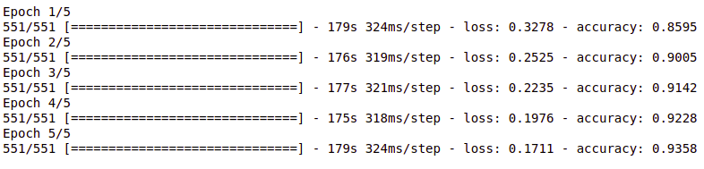
history = model.fit(train_pad,
                    y_train,
                    epochs=5)

Output:

Training Process of the SimpleRNN model

Extra: RNN Gated Cells Architecture

Recurrent Neural Networks are the hardest to train. Since this Neural Network is pruned to Vanishing Gradients. To overcome this issue, many researchers worked to develop a better version of RNN. Some solution provided to Vanishing gradients is to include a proper activation function that can prevent the shrinking of the gradients. The next solution is the initialization of weights and biases. One another method is using complex gated cells. Example of these complex gated cells is LSTM and GRU. This architecture consists of a separate cell state and forger gate that allows information to pass through unchanged. 

We shall now train LSTM(Long Short Term Memory) and GRU(Gated Recurrent Unit) Recurrent Neural Network architecture in TensorFlow. 

Bidirectional LSTM and GRU

The bidirectional layer is mainly used when you have a feedback network, in this case, Bidirectional LSTM is the process of making a Neural Network have the sequence of data in both directions i.e., forwards (past to future) and backward (future to past). Since RNN backpropagate back to a time, Birecdirectional LSTM or GRU ar

Python3

model = keras.models.Sequential()
model.add(keras.layers.Embedding(10000, 128))
model.add(keras.layers.Bidirectional(
    keras.layers.LSTM(64, return_sequences=True)))
model.add(keras.layers.Bidirectional(keras.layers.LSTM(64)))
model.add(keras.layers.Dense(128, activation="relu"))
model.add(keras.layers.Dropout(0.4))
model.add(keras.layers.Dense(1, activation="sigmoid"))

model.compile("rmsprop", "binary_crossentropy", metrics=["accuracy"])
history = model.fit(train_pad, y_train, epochs=5)

Output:

Training Process of the Bidirectional LSTM model

Now let’s check the model’s accuracy using GRUs as well.

Python3

model = keras.models.Sequential()
model.add(keras.layers.Embedding(10000, 128))
model.add(keras.layers.Bidirectional(
    keras.layers.GRU(64, return_sequences=True)))
model.add(keras.layers.Bidirectional(keras.layers.GRU(64)))
model.add(keras.layers.Dense(128, activation="relu"))
model.add(keras.layers.Dropout(0.4))
model.add(keras.layers.Dense(1, activation="sigmoid"))

model.compile("rmsprop", "binary_crossentropy", metrics=["accuracy"])
history = model.fit(train_pad, y_train, epochs=5)

Output:

Training Process of the GRU model

If you notice the accuracy difference, the model performed better in LSTM and GRU cases than in simpler ones. We shall conclude this article by discussing the applications, where RNNs are used widely.