TOPSIS method for Multiple-Criteria Decision Making (MCDM)
Last Updated :
05 Oct, 2021
Technique for Order Preference by Similarity to Ideal Solution (TOPSIS) came in the 1980s as a multi-criteria-based decision-making method. TOPSIS chooses the alternative of shortest the Euclidean distance from the ideal solution and greatest distance from the negative ideal solution.
To make this definition easier, let’s suppose you want to buy a mobile phone, you go to a shop and analyze 5 mobile phones on basis of RAM, memory, display size, battery, and price. At last, you’re confused after seeing so many factors and don’t know how to decide which mobile phone you should purchase. TOPSIS is a way to allocate the ranks on basis of the weights and impact of the given factors.
- Weights mean how much a given factor should be taken into consideration (default weight = 1 for all factors). like you want RAM to have weighed more than other factors, so the weight of RAM can be 2, while others can have 1.
- Impact means that a given factor has a positive or negative impact. Like you want Battery to be large as possible but the price of the mobile to be less as possible, so you’ll assign ‘+’ weight to the battery and ‘-‘ weight to the price.
This method can be applied in ranking machine learning models on basis of various factors like correlation, R^2, accuracy, Root mean square error, etc. Now that we have understood what is TOPSIS, and where we can apply this. Let’s see what is the procedure to implement TOPSIS on a given dataset, consisting of multiple rows (like various mobile phones) and multiple columns (like various factors).
Example of dataset:
Given data values for a particular factor is to be considered as standard units. Always LabelEncode any non-numeric datatype.

Procedure:
Step 1: Calculating Normalized Matrix and weighted Normalize matrix. We normalize each value by making it: where m is the number of rows in the dataset and n is the number of columns. I vary along rows and j varies along the column.

Normalized matrix for the above-given values will be:
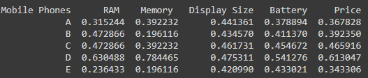
We then multiply each value in a column with the corresponding weight given.
# Arguments are dataset, number of columns, and weights of each column
def Normalize(dataset, nCol, weights):
    for i in range(1, nCol):
        temp = 0
        # Calculating Root of Sum of squares of a particular column
        for j in range(len(dataset)):
            temp = temp + dataset.iloc[j, i]**2
        temp = temp**0.5
        # Weighted Normalizing a element
        for j in range(len(dataset)):
            dataset.iat[j, i] = (dataset.iloc[j, i] / temp)*weights[i-1]
    print(dataset)
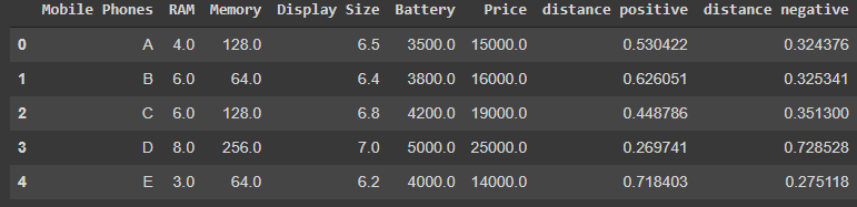
Step 2: Calculating Ideal Best and Ideal worst and Euclidean distance for each row from ideal worst and ideal best value. First, we will find out the ideal best and ideal worst value: Now here we need to see the impact, i.e. is it ‘+’ or ‘-‘ impact. If ‘+’ impact Ideal best for a column is the maximum value in that column and the ideal worst is the minimum value in that column, and vice versa for the ‘-‘ impact.
# Calculate ideal best and ideal worst
def Calc_Values(dataset, nCol, impact):
    p_sln = (dataset.max().values)[1:]
    n_sln = (dataset.min().values)[1:]
    for i in range(1, nCol):
        if impact[i-1] == '-':
            p_sln[i-1], n_sln[i-1] = n_sln[i-1], p_sln[i-1]
    return p_sln, n_sln
Now we need to calculate Euclidean distance for elements in all rows from the ideal best and ideal worst, Here diw is the worst distance calculated of an ith row, where ti,j is element value and tw,j is the ideal worst for that column. similarly, we can find dib, i.e. best distance calculated on an ith row.

Now the dataset will look something like this with the positive and negative distance included.
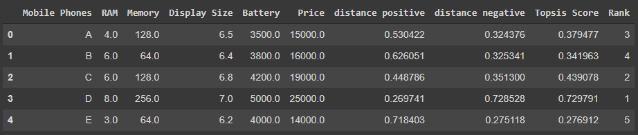
Step 3: Calculating Topsis Score and Ranking. Now we have Distance positive and distance negative with us, let’s calculate the Topsis score for each row on basis of them.
TOPSIS Score = diw / (dib + diw) for each row
Now rank according to the TOPSIS score, i.e. higher the score, better the rank
Our dataset will be ranked like this:
Code for the last part is here!
 # Calculating positive and negative values
 p_sln, n_sln = Calc_Values(temp_dataset, nCol, impact)

 # calculating topsis score
 score = [] # Topsis score
 pp = [] # distance positive
 nn = [] # distance negative


# Calculating distances and Topsis score for each row
 for i in range(len(temp_dataset)):
     temp_p, temp_n = 0, 0
     for j in range(1, nCol):
         temp_p = temp_p + (p_sln[j-1] - temp_dataset.iloc[i, j])**2
         temp_n = temp_n + (n_sln[j-1] - temp_dataset.iloc[i, j])**2
     temp_p, temp_n = temp_p**0.5, temp_n**0.5
     score.append(temp_n/(temp_p + temp_n))
     nn.append(temp_n)
     pp.append(temp_p)

 # Appending new columns in dataset

 dataset['distance positive'] = pp
 dataset['distance negative'] = nn
 dataset['Topsis Score'] = score

 # calculating the rank according to topsis score
 dataset['Rank'] = (dataset['Topsis Score'].rank(method='max', ascending=False))
 dataset = dataset.astype({"Rank": int})
You can find Code Source on my Github Repo: Link
Like Article
Suggest improvement
Share your thoughts in the comments
Please Login to comment...