Ted Talks Recommendation System with Machine Learning

When did we see a video on youtube let’s say it was funny then the next time you open your youtube app you get recommendations of some funny videos in your feed ever thought about how? This is nothing but an application of Machine Learning using which recommender systems are built to provide personalized experience and increase customer engagement.

In this article, we will try to build a very basic recommender system that can recommend ted talks based on what are the topics of your interest.

Importing Libraries & Dataset

Python libraries make it very easy for us to handle the data and perform typical and complex tasks with a single line of code.

• Pandas – This library helps to load the data frame in a 2D array format and has multiple functions to perform analysis tasks in one go.
• Numpy – Numpy arrays are very fast and can perform large computations in a very short time.
• MatplotLib/Wordcloud – This library is used to draw visualizations.
• nltk – This library is used to perform text processing on the raw text data.

Python3

%%capture
import numpy as np
import pandas as pd
import matplotlib.pyplot as plt

import nltk
import string
import warnings
from scipy.stats import pearsonr
from nltk.corpus import stopwords
from wordcloud import WordCloud
from sklearn.feature_extraction.text import TfidfVectorizer
from sklearn.metrics.pairwise import cosine_similarity

nltk.download('stopwords')
warnings.filterwarnings('ignore')

The dataset we are going to use contains data about Ted talks that happened in the span of years 2006 – 2020. Along with the name of the speaker and the main title of those Ted Talks.

Python3

df = pd.read_csv('tedx_dataset.csv')
print(df.head())

Output:

First five rows of the dataset

Python3

df.shape

Output:

 (4467, 9)

Now let’s check if there are null values present in the dataset.

Python3

df.isnull().sum()

Output:

Sum of null values column-wise

Here we can see that almost 95% of the data is missing from the num_views columns so, we won’t be able to derive any insights from this column of the data.

Python3

splitted = df['posted'].str.split(' ', expand=True)

# Creating columns for month and year of the talk
df['year'] = splitted[2].astype('int')
df['month'] = splitted[1]

Now let’s check what is the trend in the number of ted talks happening yearly.

Python3

df['year'].value_counts().plot.bar()
plt.show()

Output:

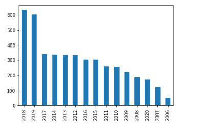
Countplot for the number of ted talks released on yearly basis.

Here we can see an approximately increasing trend in the number of ted talks released on the yearly basis except for some exceptions.

Python3

# Let's combine the title and the details of the talk.
df['details'] = df['title'] + ' ' + df['details']

# Removing the unnecessary information
df = df[['main_speaker', 'details']]
df.dropna(inplace = True)
df.head()

Output:

Python3

# We would like to have a copy of our data for future use.
data = df.copy()

Text Preprocessing

In general data we obtained in the form of raw text requires a lot of preprocessing before it can be used to develop any model. Removal of stopwords, stemming, lemmatization, and removing punctuations are some steps that help us to convert the raw textual data into a usable format.

Python3

def remove_stopwords(text):
  stop_words = stopwords.words('english')

  imp_words = []

  # Storing the important words
  for word in str(text).split():
    word = word.lower()

    if word not in stop_words:
      imp_words.append(word)

  output = " ".join(imp_words)

  return output

Now, let’s use the above helper function to remove the stopwords present in our data.

Python3

df['details'] = df['details'].apply(lambda text: remove_stopwords(text))
df.head()

Output:

Now, we will remove any punctuations present in the data.

Python3

punctuations_list = string.punctuation


def cleaning_punctuations(text):
    signal = str.maketrans('', '', punctuations_list)
    return text.translate(signal)


df['details'] = df['details'].apply(lambda x: cleaning_punctuations(x))
df.head()

Output:

WordCloud is a visualization tool that helps us to visualize the occurrence of words. Like which are the words that are more frequent in our text corpus.

Python3

details_corpus = " ".join(df['details'])

plt.figure(figsize=(20, 20))
wc = WordCloud(max_words=1000,
               width=800,
               height=400).generate(details_corpus)
plt.axis('off')
plt.imshow(wc)
plt.show()

Output:

WordCloud of the text corpus

From the above word cloud, we can observe that words like world, help, people, life, help are some of the most frequent words. This seems like aligning with the objective of ted talks which is to help this world through the experiences of some successful people.

Recommender System

As the details are all that we have about the talks we will use them to build our recommender system. We will use the Tf-IDF vectorizer to convert your textual data into their numerical representations.

Python

%%capture
vectorizer = TfidfVectorizer(analyzer = 'word')
vectorizer.fit(df['details'])

We will use two types of indicators to measure the similarity between our data and the input by the user:

1. Cosine Similarity – This is a useful metric to measure the similarity between the two objects.
2. Pearson Correlation – Pearson’s correlation coefficient formula is the most commonly used and the most popular formula to get the correlation coefficient.

Python3

def get_similarities(talk_content, data=df):

    # Getting vector for the input talk_content.
    talk_array1 = vectorizer.transform(talk_content).toarray()

    # We will store similarity for each row of the dataset.
    sim = []
    pea = []
    for idx, row in data.iterrows():
        details = row['details']

        # Getting vector for current talk.
        talk_array2 = vectorizer.transform(
            data[data['details'] == details]['details']).toarray()

        # Calculating cosine similarities
        cos_sim = cosine_similarity(talk_array1, talk_array2)[0][0]

        # Calculating pearson correlation
        pea_sim = pearsonr(talk_array1.squeeze(), talk_array2.squeeze())[0]

        sim.append(cos_sim)
        pea.append(pea_sim)

    return sim, pea

The below function will call the above helper function to get the similarity between the input and the data of the talk we have.

Python3

def recommend_talks(talk_content, data=data):

    data['cos_sim'], data['pea_sim'] = get_similarities(talk_content)

    data.sort_values(by=['cos_sim', 'pea_sim'], ascending=[
                     False, False], inplace=True)

    display(data[['main_speaker', 'details']].head())

Now, it’s time to see the recommender system at work. Let’s see which talks are recommended by the system based on the different major topics which revolve around the world.

Python3

talk_content = ['Time Management and working\
hard to become successful in life']
recommend_talks(talk_content)

Output:

Let’s look at one more example.

Python3

talk_content = ['Climate change and impact on the health\
. How can we change this world by reducing carbon footprints?']
recommend_talks(talk_content)

Output: