Support Vector Machine (SVM) Algorithm
Last Updated :
10 Jun, 2023
Support Vector Machine (SVM) is a powerful machine learning algorithm used for linear or nonlinear classification, regression, and even outlier detection tasks. SVMs can be used for a variety of tasks, such as text classification, image classification, spam detection, handwriting identification, gene expression analysis, face detection, and anomaly detection. SVMs are adaptable and efficient in a variety of applications because they can manage high-dimensional data and nonlinear relationships.
SVM algorithms are very effective as we try to find the maximum separating hyperplane between the different classes available in the target feature.
Support Vector Machine
Support Vector Machine (SVM) is a supervised machine learning algorithm used for both classification and regression. Though we say regression problems as well it’s best suited for classification. The main objective of the SVM algorithm is to find the optimal hyperplane in an N-dimensional space that can separate the data points in different classes in the feature space. The hyperplane tries that the margin between the closest points of different classes should be as maximum as possible. The dimension of the hyperplane depends upon the number of features. If the number of input features is two, then the hyperplane is just a line. If the number of input features is three, then the hyperplane becomes a 2-D plane. It becomes difficult to imagine when the number of features exceeds three.
Let’s consider two independent variables x1, x2, and one dependent variable which is either a blue circle or a red circle.
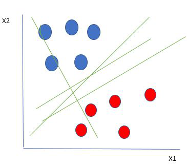
Linearly Separable Data points
From the figure above it’s very clear that there are multiple lines (our hyperplane here is a line because we are considering only two input features x1, x2) that segregate our data points or do a classification between red and blue circles. So how do we choose the best line or in general the best hyperplane that segregates our data points?
How does SVM work?
One reasonable choice as the best hyperplane is the one that represents the largest separation or margin between the two classes.
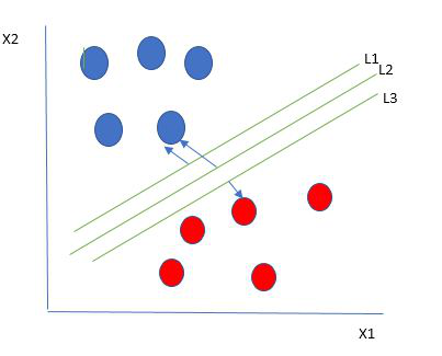
Multiple hyperplanes separate the data from two classes
So we choose the hyperplane whose distance from it to the nearest data point on each side is maximized. If such a hyperplane exists it is known as the maximum-margin hyperplane/hard margin. So from the above figure, we choose L2. Let’s consider a scenario like shown below
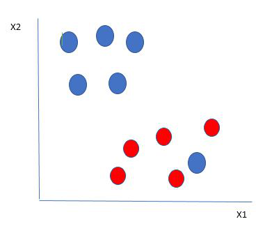
Selecting hyperplane for data with outlier
Here we have one blue ball in the boundary of the red ball. So how does SVM classify the data? It’s simple! The blue ball in the boundary of red ones is an outlier of blue balls. The SVM algorithm has the characteristics to ignore the outlier and finds the best hyperplane that maximizes the margin. SVM is robust to outliers.
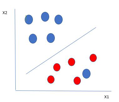
Hyperplane which is the most optimized one
So in this type of data point what SVM does is, finds the maximum margin as done with previous data sets along with that it adds a penalty each time a point crosses the margin. So the margins in these types of cases are called soft margins. When there is a soft margin to the data set, the SVM tries to minimize (1/margin+∧(∑penalty)). Hinge loss is a commonly used penalty. If no violations no hinge loss.If violations hinge loss proportional to the distance of violation.
Till now, we were talking about linearly separable data(the group of blue balls and red balls are separable by a straight line/linear line). What to do if data are not linearly separable?
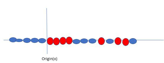
Original 1D dataset for classification
Say, our data is shown in the figure above. SVM solves this by creating a new variable using a kernel. We call a point xi on the line and we create a new variable yi as a function of distance from origin o.so if we plot this we get something like as shown below
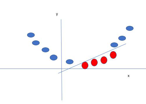
Mapping 1D data to 2D to become able to separate the two classes
In this case, the new variable y is created as a function of distance from the origin. A non-linear function that creates a new variable is referred to as a kernel.
Support Vector Machine Terminology
- Hyperplane: Hyperplane is the decision boundary that is used to separate the data points of different classes in a feature space. In the case of linear classifications, it will be a linear equation i.e. wx+b = 0.
- Support Vectors: Support vectors are the closest data points to the hyperplane, which makes a critical role in deciding the hyperplane and margin.
- Margin: Margin is the distance between the support vector and hyperplane. The main objective of the support vector machine algorithm is to maximize the margin. The wider margin indicates better classification performance.
- Kernel: Kernel is the mathematical function, which is used in SVM to map the original input data points into high-dimensional feature spaces, so, that the hyperplane can be easily found out even if the data points are not linearly separable in the original input space. Some of the common kernel functions are linear, polynomial, radial basis function(RBF), and sigmoid.
- Hard Margin: The maximum-margin hyperplane or the hard margin hyperplane is a hyperplane that properly separates the data points of different categories without any misclassifications.
- Soft Margin: When the data is not perfectly separable or contains outliers, SVM permits a soft margin technique. Each data point has a slack variable introduced by the soft-margin SVM formulation, which softens the strict margin requirement and permits certain misclassifications or violations. It discovers a compromise between increasing the margin and reducing violations.
- C: Margin maximisation and misclassification fines are balanced by the regularisation parameter C in SVM. The penalty for going over the margin or misclassifying data items is decided by it. A stricter penalty is imposed with a greater value of C, which results in a smaller margin and perhaps fewer misclassifications.
- Hinge Loss: A typical loss function in SVMs is hinge loss. It punishes incorrect classifications or margin violations. The objective function in SVM is frequently formed by combining it with the regularisation term.
- Dual Problem: A dual Problem of the optimisation problem that requires locating the Lagrange multipliers related to the support vectors can be used to solve SVM. The dual formulation enables the use of kernel tricks and more effective computing.
Mathematical intuition of Support Vector Machine
Consider a binary classification problem with two classes, labeled as +1 and -1. We have a training dataset consisting of input feature vectors X and their corresponding class labels Y.
The equation for the linear hyperplane can be written as:

The vector W represents the normal vector to the hyperplane. i.e the direction perpendicular to the hyperplane. The parameter b in the equation represents the offset or distance of the hyperplane from the origin along the normal vector w.
The distance between a data point x_i and the decision boundary can be calculated as:

where ||w|| represents the Euclidean norm of the weight vector w. Euclidean norm of the normal vector W
For Linear SVM classifier :

Optimization:
- For Hard margin linear SVM classifier:

The target variable or label for the ith training instance is denoted by the symbol ti in this statement. And ti=-1 for negative occurrences (when yi= 0) and ti=1positive instances (when yi = 1) respectively. Because we require the decision boundary that satisfy the constraint: 
- For Soft margin linear SVM classifier:

- Dual Problem: A dual Problem of the optimisation problem that requires locating the Lagrange multipliers related to the support vectors can be used to solve SVM. The optimal Lagrange multipliers α(i) that maximize the following dual objective function

where,
- αi is the Lagrange multiplier associated with the ith training sample.
- K(xi, xj) is the kernel function that computes the similarity between two samples xi and xj. It allows SVM to handle nonlinear classification problems by implicitly mapping the samples into a higher-dimensional feature space.
- The term ∑αi represents the sum of all Lagrange multipliers.
The SVM decision boundary can be described in terms of these optimal Lagrange multipliers and the support vectors once the dual issue has been solved and the optimal Lagrange multipliers have been discovered. The training samples that have i > 0 are the support vectors, while the decision boundary is supplied by:

Types of Support Vector Machine
Based on the nature of the decision boundary, Support Vector Machines (SVM) can be divided into two main parts:
- Linear SVM: Linear SVMs use a linear decision boundary to separate the data points of different classes. When the data can be precisely linearly separated, linear SVMs are very suitable. This means that a single straight line (in 2D) or a hyperplane (in higher dimensions) can entirely divide the data points into their respective classes. A hyperplane that maximizes the margin between the classes is the decision boundary.
- Non-Linear SVM: Non-Linear SVM can be used to classify data when it cannot be separated into two classes by a straight line (in the case of 2D). By using kernel functions, nonlinear SVMs can handle nonlinearly separable data. The original input data is transformed by these kernel functions into a higher-dimensional feature space, where the data points can be linearly separated. A linear SVM is used to locate a nonlinear decision boundary in this modified space.
Popular kernel functions in SVM
The SVM kernel is a function that takes low-dimensional input space and transforms it into higher-dimensional space, ie it converts nonseparable problems to separable problems. It is mostly useful in non-linear separation problems. Simply put the kernel, does some extremely complex data transformations and then finds out the process to separate the data based on the labels or outputs defined.

Advantages of SVM
- Effective in high-dimensional cases.
- Its memory is efficient as it uses a subset of training points in the decision function called support vectors.
- Different kernel functions can be specified for the decision functions and its possible to specify custom kernels.
SVM implementation in Python
Predict if cancer is Benign or malignant. Using historical data about patients diagnosed with cancer enables doctors to differentiate malignant cases and benign ones are given independent attributes.
Steps
- Load the breast cancer dataset from sklearn.datasets
- Separate input features and target variables.
- Buil and train the SVM classifiers using RBF kernel.
- Plot the scatter plot of the input features.
- Plot the decision boundary.
- Plot the decision boundary
Python3
from sklearn.datasets import load_breast_cancer
import matplotlib.pyplot as plt
from sklearn.inspection import DecisionBoundaryDisplay
from sklearn.svm import SVC
cancer = load_breast_cancer()
X = cancer.data[:, :2]
y = cancer.target
svm = SVC(kernel="rbf", gamma=0.5, C=1.0)
svm.fit(X, y)
DecisionBoundaryDisplay.from_estimator(
svm,
X,
response_method="predict",
cmap=plt.cm.Spectral,
alpha=0.8,
xlabel=cancer.feature_names[0],
ylabel=cancer.feature_names[1],
)
plt.scatter(X[:, 0], X[:, 1],
c=y,
s=20, edgecolors="k")
plt.show()
|
Output:
.png)
Breast Cancer Classifications with SVM RBF kernel
Like Article
Suggest improvement
Share your thoughts in the comments
Please Login to comment...