Sparse Transformer: Stride and Fixed Factorized Attention

Last Updated : 16 Mar, 2021

Strided and Fixed attention were proposed by researchers @ OpenAI in the paper called ‘Generating Long Sequences with Sparse Transformers ‘. They argue that Transformer is a powerful architecture, However, it has the quadratic computational time and space w.r.t the sequence length. So, this inhibits the ability to use large sequences. That’s why they also propose a new Sparse transformer, which reduces the time complexity to O(n^(1+1/p)) where p>1 (p ~=2) by making some changes in Transformer architecture,

They also made some changes in the residual block and weight initialization method to improve the training of deep networks.
To compute the attention matrix in a faster and efficient way, they also introduced a set of sparse kernels that computes the subset of it efficiently.

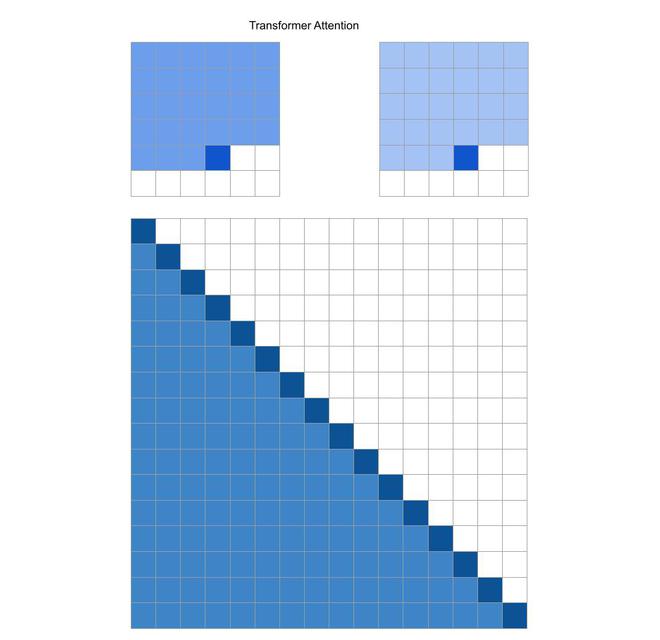
Standard Transformer

In the figure above, a standard transformer processing an image of 6×6 and 2 attention heads. The above row indicates a 6×6 image, which positions two attention heads receive as input when computing a given output. The bottom row indicates connectivity matrix b/w all such outputs(rows) and inputs(columns). We will follow this convention in future images as well.

Architecture:

Let’s consider an auto regressive sequence generation problem, where the joint probability of a distribution x ={x₁,x₂,..x_n} is the product of conditional probability, parameterized by $\theta$

$p(x) = \prod_{i=1}^{n} p(x_i | x_1,x_2,x_3 ...x_{i-1} ; \theta)$

Here, images, audio, video can also be treated as a sequence of raw bytes.

The network takes on the sequence input and outputs a categorical distribution over v, where v is the size of vocabulary which is obtained after softmax on output of network \theta.

A good choice for this type of model is Transformer. However, Transformer requires computing self-attention matrix which requires O(n²) computability. Hence, the authors of this paper made some modifications to the transformer architecture. Let’s discuss these modifications in detail.

Factorized Self attention:

A self-attention matrix maps an input embedding to output matrix and its parameterized by the connectivity pattern

$S = \left \S_1,S_2, ..., S_n{ \right \}$

where, S_i denote the set of indices of input vector to which the i^th output vector attends. Self-attention can be expressed by the following expression:

$Attend \left ( X,S \right ) = a\left ( a(x_i, S_i)\right )_{\left \{ i \epsilon i_1, i_2 ....i_n \right \}} \\ \\ a(x_i,S_i) = softmax(\frac{(W_q x_i) K_{S_i}^{T} }{\sqrt(d)}V_{S_i}) \\ \\ K_{S_i} = \left ( W_k x_j \right )_{j \epsilon S_i} \\ \\V_{S_i} = \left ( W_V x_j \right )_{j \epsilon S_i}$

where, W_q, W_k W_v are the weights ,

Instead of attending all the previous values before predicting the current value, the authors tries to perform it more efficiently by dividing all the attention heads into p separate attention heads, where m^th head defines the subset of indices A_i^(m) A_i^(m) A_i^{(m)} \subset {j: j \leq i} and lets S_i =A_i^{(m)}. The goal of the author is to divide the attention heads into efficient subset so that

$\left |A_i^{(m)} \right | \propto \sqrt[p]{n}$

Additionally, the author looked for choices of A such that so that all inputs are connected to all future output positions across the p attention steps.

For every pair j<=i, the authors set every A such that i can attend to j through a path of locations with maximum length p+1.

$j \epsilon A_{a}^{(1)} ; a \epsilon A_{b}^{(2)}; b \epsilon A_{c}^{(3)}$

Two-dimensional Factorized Attention:

Strided Attention:

One of the approach of predicting the current pixel in two-dimensional is that the one head attends to l previous pixel and other head attends to every l^th location where l is called stride, and it’s value is chosen to be \sqrt{n}. In this pattern, the first head attends

The stride attention can be represented by the following equations:

$A_i^{1} = \left \{ t, t+1, ... i \right \} ; for \, t = max\left ( 0,i-l \right ) \\ A_i^{2} = \left \{ j: \left ( i-j \right ) mod \, \, l =0 \right \}$

This pattern of attention works when data inherently has some kind of pattern that aligns with the stride like images data and music data. This won’t work for dataset which didn’t contain any periodic pattern and fail to communicate information b/w attention head.

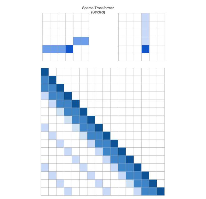
Sparse Transformer (strided)

Fixed Attention:

In the case where there is a lack of structure and periodicity in the data, the authors propose a method for two-dimensional factorization called fixed attention, where specific cells summarize the previous locations and propagate the information to all future cells. This can be mathematically represented by the following equations: $attention(X) = W_p \cdot attend(X,S)$

$A_{(i)}^{1} = \left \{ j: \lfloor{\frac{j}{l}} \rfloor = \lfloor{\frac{i}{l}} \rfloor \right \}$

$A_{(i)}^{2} = \left \{ j: j mod \,\, l \, \epsilon \left \{ t, t+1 , .. l-1 \right \} \right \}$

where, t= l-c and c is hyper parameter.

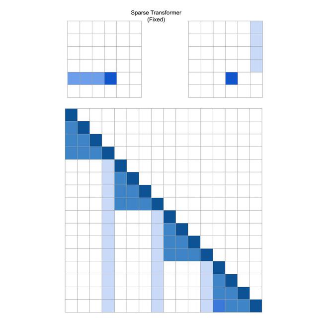
Sparse Transformer (Fixed)

Sparse Transformer:

Factorized Attention

The standard dense attention performs a linear transformation of the attend function:

$attention(X) = W_p \cdot attend(X,S)$

where, W_p is post-attention weight matrix. However, from the above methods, we know that we have more than one attention heads, so how do we integrate them. The author proposes three methods to perform this:

The most basic technique for integrating factorized self-attention is to use one type of attention per residual block and interleave them sequentially at a ratio, which can be determined by hyper parameter. The mathematical expression for this type of integration below:

$attention(X) = W_p \cdot attend(X,A^{(r\, mod \, p)})$

Here, r is the current residual block and p is a number of attention heads.

Another approach is to have a single head attend to the locations of the pixels that both factorized heads would attend to, which the authors merged head. This approach is slightly more computationally expensive.

$attention(X) = W_p \cdot attend(X,\bigcup_{m=1}^{P} \, A^{(m)})$

A third approach which is used in multi-headed attention is also used by authors most of the time. In this method,, n_h attention products are computed in parallel and concatenated along the feature dimension

$attention(X) = W_p\left ( attend(X, A)^{(i)} \right )_{i \epsilon \left \{ 1,2...,n_h \right \}} \\$

Scaling to 100 layers

The authors of this paper make some important changes in the architecture in order to make it easier to train the transformer of many layers, first they use the pre-activation block similar to residual block used in ResNet paper

$H_0 = embed(X ,W_e) \\ \\ H_k = H_{k-1} + resblock(H_{k-1}) \\ \\ Y = softmax(norm(H_N)W_{out})$

where W_outis the matrix of weights, resblock(h) normalizes the input and position wise feed forward the attention in following way:

$a(H) = dropout(attention(norm(H))) \\ b(H) = dropout(ff(norm(H + a(H)))) \\ resblock(H) = a(H) + b(H)$

Here, the norm function denotes layer normalization, and ff is an activation function, the right choice of ff is Gauss Error Linear Unit according to authors.

Modelings diverse data types

To encode the spatial relationship of the data, the Transformer mostly uses position based embedding and other location-specific architecture. The authors also concludes that position wise embedding is best for the model. The authors calculate these embeddings as follows:

$embed (X, W_e) = \left ( x_i*W_e + \sum_{j=1}^{n_{emb}}o_{i}^{(j)}*W_j \right )_{x_i \epsilon X}$

Where n_emb = d_data(dimension of data) or n_emb = d_attn(dimension of attention). For the image data, the n_emb =3 (d_data =3 width* height* channels), for the text and audio data, n_emb =2 because d_attn =2 and the index here corresponds to each position’s row and column index in a matrix of width equal to the stride. Here, x_i is the one-hot encoded i^th element in the sequence, and o_i^(j) represents the one-hot encoded position of x_iin j^th dimension.

Saving memory by recomputing attention weights

Gradient checkpointing was the technique devised by OpenAI researchers that let users fit 10x bigger models into the GPU at the cost of 20% extra computations. It is particularly effective for training self-attention layers when long sequences are processed as they require high memory uses.

Using recomputation only, the authors are able to fit a sequence of length 16,384 (2^14) with 100s of the layer which would be otherwise infeasible even with modern architecture.

Efficient block-sparse attention kernels:

The sparse attention masks for strided and fixed attention can be computed by slicing-out parts of the queries, keys and values matrices and computing the product in blocks. Moreover, the upper triangle of the attention matrix is never computed, reducing the number of operations to half.

Mixed-precision training

The network weights are stored in single-precision floating-point, but, network activation and gradients are computed in half-precision. This helps us accelerate the model training on Nvidia V100 GPU.

References

Sparse Transformer paper

Suggest improvement

Introduction to Speech Separation Based On Fast ICA

Wine Quality Prediction - Machine Learning

Share your thoughts in the comments