Solving Linear Regression without using Sklearn and TensorFlow

In this article, we will see how can we implement a Linear Regression class on our own without using any of the sklearn or the Tensorflow API pre-implemented functions which are highly optimized for such tasks. But then why we are implementing these functions on our own? The answer to this is very simple that is because they help to clarify our concept of how to implement an idea in code.

Importing Libraries and Dataset

Python libraries make it easy for us to handle the data and perform typical and complex tasks with a single line of code.

• Pandas – This library helps to load the data frame in a 2D array format and has multiple functions to perform analysis tasks in one go.
• Numpy – Numpy arrays are very fast and can perform large computations in a very short time.

Python3

import numpy as np
import pandas as pd
import matplotlib.pyplot as plt

We will be using the salary dataset here which contains only two columns having years of experience as a feature column and salary as a target column.

Python3

df = pd.read_csv('Salary_Data.csv')
df.head()

Output:

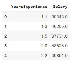
First five rows of the dataset

Python3

df.shape

Output:

(30, 2)

Although the dataset is small it is good for demonstration purposes.

Python3

X = df['YearsExperience'].values.reshape(-1, 1)
Y = df['Salary'].values.reshape(-1, 1)

Linear Regression

Now we will implement a LinearRegression class which will contain multiple functions which will be used for the gradient descent, updating parameters, and obtaining the trained final weights.

Python3

class Linear_Regression():

    # Initiating the parameters.
    def __init__(self, learning_rate, no_of_itr):
        self.learning_rate = learning_rate
        self.no_of_itr = no_of_itr

    def fit(self, X, Y):

        # No. of training examples and no. of features.
        self.m, self.n = X.shape     # Number of rows and columns
        # Initiating the weight and bias
        self.w = np.zeros((self.n, 1))
        self.b = 0
        self.X = X
        self.Y = Y

        # Implementing the gradient descent.
        for i in range(self.no_of_itr):
            self.update_weigths()

    def update_weigths(self):
        Y_prediction = self.predict(self.X)

        # Calculating gradients
        dw = -(self.X.T).dot(self.Y - Y_prediction)/self.m

        db = -np.sum(self.Y - Y_prediction)/self.m

        # Updating weights
        self.w = self.w - self.learning_rate * dw
        self.b = self.b - self.learning_rate * db

    def predict(self, X):
        return X.dot(self.w) + self.b

    def print_weights(self):
        print('Weights for the respective features are :')
        print(self.w)
        print()

        print('Bias value for the regression is ', self.b)

Let’s create an object of the above class and train it for 2000 iterations with a learning rate of 0.03.

Python3

model = Linear_Regression(learning_rate=0.03,
                          no_of_itr=2000)
model.fit(X_train, Y_train)

Now let’s check the model weights which are optimized by using the gradient descent algorithm.

Python3

model.print_weights()

Output:

Weights for the respective features are :
[[9988.54665892]]

Bias value for the regression is  23876.191228516196

Plotting the line obtained and the along with the points will help us to visualize whether the trained weights of the Linear Regression are optimal or not.

Python3

plt.scatter(df['YearsExperience'], df['Salary'])
plt.xlabel('Years of Experience')
plt.ylabel('Salary')
plt.title('Exp v/s Salary')

X = df['YearsExperience'].values
plt.plot(X, 9988 * X + 23876)
plt.show()

Output:

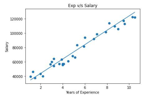
Visualizing the line and the points using a scatter plot

This is quite an accurate line for the dataset we have used here. This implies that the LinearRegression model we have used here is quite accurate.