Singular Value Decomposition

Last Updated : 29 Mar, 2023

Prerequisites: Matrix Diagonalization, Eigenvector Computation and Low-Rank Approximations

Before getting in depth into the SVD, let us first briefly understand what Matrix Diagonalization technique is and when it fails to perform efficiently.

Matrix Diagonalization

Matrix diagonalization is the process of taking a square matrix and converting it into a special type of matrix known as the diagonal matrix. This matrix shares the same fundamental properties of the underlying matrix. Mathematically, any input matrix A can be reduced into any diagonal matrix D if it satisfies:

$D = P ^{-1} A P$

where,
P -> Modal Matrix: It is a (n x n) matrix that consists of eigen-vectors. 
               It is generally used in the process of diagonalization 
               and similarity transformation.

However, the matrix diagonalization technique fails for matrices of the form (m x n) where m ≠ n. (i.e. when the matrix is not a square matrix. This is where ‘Singular Value Decomposition’ comes into picture and provides a good solution to this problem.

Singular Values (σ)

Let A be any m x n matrix with rank r. On multiply it with its transpose (i.e. A^TA), a n x n matrix is created which is symmetric as well as positive semi-definite in nature. In simpler terms, all the Eigen values (λ_i…r) of A^TA matrix are non-negative (i.e. greater than 0).

The singular values are defined as the square root of the obtained Eigen values. That is:

$\sigma_i = \sqrt{\lambda_i} \\ where \ (i \le r)$

Singular Value Decomposition (SVD)

Let A be any m x n matrix. Then the SVD divides this matrix into 2 unitary matrices that are orthogonal in nature and a rectangular diagonal matrix containing singular values till r. Mathematically, it is expressed as:

$A = U \Sigma V^T$

where, 
Σ -> (m x n) diagonal matrix where the elements of the diagonal are the singular values
U -> (m x m) orthogonal matrix whose columns are the left singular vectors
V -> (n x n) orthogonal matrix whose columns are the right singular vectors

Now, It is important to understand how to calculate the matrices U, V & Σ.

Calculating normalized eigeinvectors

First, we calculate the Eigen vectors x_i associated of a square matrix X. Then, we find the normalized eiegnvectors v_i corresponding to the eigenvectors x_iby dividing each value in vector x_iby its magnitude. For example:

Let x = [1,2,4]
=> mag(x) or |x| = √(1² + 2² + 4²) = √21.

Therefore, v = [(1/√21), (2/√21), (4/√21)]

Calculating orthogonal matrix V

We know, A is a m x n matrix. Therefore, A^TA is a n x n symmetric matrix with all Eigen values > 0. So, we can obtain Eigen vectors v_1…nof A^TA such that:

$(A^TA)v_i = \sigma_i^2v_i = \lambda_iv_i$

where,
x_{i ->} eigen vector
v_{i ->} normalized eigen vector.
and
σ_{i ->} corresponding singular value.
λ_{i ->} corresponding eigen value.

Upon calculating the Eigen vectors of AAT, matrix V will be:

$V = \begin{bmatrix} v_1 & v_2 & ...\ v_i\end{bmatrix}$

where, v₁, v₂, ... v_i are arranged column-wise into matrix V.

Calculating orthogonal matrix U

Similarly, for any A (m x n) matrix, AA^T is a m x m symmetric matrix with all eigen values > 0. So, we can obtain eigen vectors x_1…n of AA^T such that:

$(AA^T)x_i = \sigma_i^2x_i = \lambda_ix_i$

where,
x_{i ->} eigen vector.
and
σ_{i ->} corresponding singular value.
λ_{i ->} corresponding eigen value.

Now, we use the following equation to compute matrix U:

$u_i = \frac{Av_i}{\sigma_i}$

Upon calculating, matrix U will be:

$U = \begin{bmatrix} u_1 & u_2 & ...\ u_i\end{bmatrix}$

where, u₁, u₂, ... u_i are arranged column-wise into matrix U.

Calculating diagonal matrix Σ

Here, matrix A has rank(A) = r where r ≤ min (m,n).

Case 1: If m ≤ n, say m = 2 & n = 4, then assuming all (σ_i> 0), Σ can be expressed as:

$\begin{bmatrix} \sigma_1 & 0 & 0 & 0\\ 0 & \sigma_2 & 0 & 0\\ \end{bmatrix}$

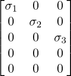
Case 2: If m ≥ n, say m = 5 & n = 3, then assuming all (σ_i > 0), Σ can be expressed as:

$\begin{bmatrix} \sigma_1 & 0 & 0 \\ 0 & \sigma_2 & 0 \\ 0 & 0 & \sigma_3 \\ 0 & 0 & 0 \\ 0 & 0 & 0 \end{bmatrix}$

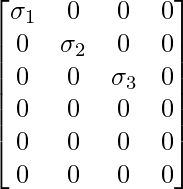
Special Case: When rank of matrix is specified, say r = 3, m = 6 & n = 4. Then Σ can be expressed as:

$\begin{bmatrix} \sigma_1 & 0 & 0 & 0\\ 0 & \sigma_2 & 0 & 0\\ 0 & 0 & \sigma_3 & 0\\ 0 & 0 & 0 & 0\\ 0 & 0 & 0 & 0\\ 0 & 0 & 0 & 0 \end{bmatrix}$

This implies that σ₄ ≤ 0, hence discarded.

NOTE: The number of singular values where σ_i > 0 can determine the rank of the matrix.

Example Problem

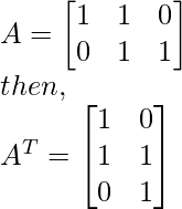
Consider the following problem. Find the SVD of a (2 x 3) matrix A having values:

$A =\begin{bmatrix} 1 & 1 & 0\\ 0 & 1 & 1\\ \end{bmatrix}$

Solution

Let us understand each step required for solving such problems.

Step 1 - Find A^T and then compute A^TA.

$A = \begin{bmatrix} 1 & 1 & 0\\ 0 & 1 & 1\\ \end{bmatrix} \\ then, \\ A^T = \begin{bmatrix} 1 & 0 \\ 1 & 1 \\ 0 & 1 \\ \end{bmatrix}$

$A^TA = \begin{bmatrix} 1 & 0 \\ 1 & 1 \\ 0 & 1 \\ \end{bmatrix} \begin{bmatrix} 1 & 1 & 0\\ 0 & 1 & 1\\ \end{bmatrix} = \begin{bmatrix} 1 & 1 & 0\\ 1 & 2 & 1\\ 0 & 1 & 1\\ \end{bmatrix}$

Step 2 - Find the eigen values associated with matrix A^TA. 
         (Discussed in the prerequisite articles mentioned above)

Eigen values associated with A^TA: λ = 0, 1 & 3.

Step 3 - Find the singular values corresponding to the obtained 
         eigen values using formula:

$\sigma_i = \sqrt{\lambda_i}$

Singular values associated with A^TA: λ = 3, 1 & 0.

λ₁ = 3 -> σ₁ = √3
λ₂ = 1 -> σ₂ = 1 
λ₃ = 0 -> σ₃ = 0

Step 4 - Compute diagonal matrix Σ using the values of σ keeping
         the above discussed cases in mind.

As (m = 2 < n = 3), Case 1 is applied and matrix Σ is:

$\Sigma = \begin{bmatrix} \sqrt{3} & 0 & 0\\ 0 & 1 & 0\\ \end{bmatrix}$

Step 5 - Find the eigen vectors & corresponding normalized eigen vectors
         associated with matrix A^TA.
         (Discussed in the prerequisite articles mentioned above)

NOTE: It is important to understand that normalized eigen vectors of A^TA define the matrix V.

Eigen vectors associated with A^TA:

For λ_{1 = 3 ->} x₁ = [1, 2, 1]
For λ_{2 = 1 ->} x₂ = [-1, 0, 1]
For λ_{3 = 0 ->} x₃ = [1, -1, 1]
 
where x₁, x₂ and x₃ are eigen vectors of matrix A^TA.

Normalized eigen vectors associated with A^TA:

For x₁ = [1, 2, 1] => v₁ = [(1/√6), (2/√6), (1/√6)]
For x₂ = [-1, 0, 1] => v₂ = [(-1/√2), 0, (1/√2)]
For x₃ = [1, -1, 1] => v₃ = [(1/√3), (-1/√3), (1/√3)]
 
where v₁, v₂ and v₃ are eigen vectors of matrix A^TA.

Step 6 - Use eigen vectors obtained to compute matrix V.

$V = \begin{bmatrix} (1/√6) & (-1/√2) & (1/√3)\\ (2/√6) & 0 & (-1/√3)\\ (1/√6) & (1/√2) & (1/√3)\\ \end{bmatrix}$

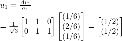
Step 7 - Use the above given equation to compute the orthogonal matrix U.

$u_1 = \frac{Av_1}{\sigma_1} \\ =\frac{1}{\sqrt{3}}\begin{bmatrix} 1 & 1 & 0\\ 0 & 1 & 1\\ \end{bmatrix}\begin{bmatrix} (1/√6) \\ (2/√6) \\ (1/√6) \\ \end{bmatrix} = \begin{bmatrix} (1/√2) \\ (1/√2) \end{bmatrix}$

$u_2 = \frac{Av_2}{\sigma_2} \\ =\frac{1}{1}\begin{bmatrix} 1 & 1 & 0\\ 0 & 1 & 1\\ \end{bmatrix}\begin{bmatrix} (-1/√2) \\ 0 \\ (1/√2) \\ \end{bmatrix} = \begin{bmatrix} (-1/√2) \\ (1/√2) \end{bmatrix}$

Therefore, orthogonal matrix U is:

$U = \begin{bmatrix} (1/√2) & (-1/√2) \\ (1/√2) & (1/√2) \end{bmatrix}$

Step 8 - Compute the SVD of A using the equation given below: 
         (As discussed above)

$A = U \Sigma V^T$

Therefore, using SVD, A can be expressed as:

$A = U \Sigma V^T \\ = \begin{bmatrix} (1/√2) & (-1/√2) \\ (1/√2) & (1/√2) \end{bmatrix} \begin{bmatrix} \sqrt{3} & 0 & 0\\ 0 & 1 & 0\\ \end{bmatrix} \begin{bmatrix} (1/√6) & (-1/√2) & (1/√3)\\ (2/√6) & 0 & (-1/√3)\\ (1/√6) & (1/√2) & (1/√3)\\ \end{bmatrix}$

Suggest improvement

Identifying handwritten digits using Logistic Regression in PyTorch

Region and Edge Based Segmentation

Share your thoughts in the comments

Singular Value Decomposition

Please Login to comment...

Similar Reads

What kind of Experience do you want to share?