Simple Linear Regression in R

Regression shows a line or curve that passes through all the data points on the target-predictor graph in such a way that the vertical distance between the data points and the regression line is minimum

What is Linear Regression?

Linear Regression is a commonly used type of predictive analysis. Linear Regression is a statistical approach for modelling the relationship between a dependent variable and a given set of independent variables. It is predicted that a straight line can be used to approximate the relationship. The goal of linear regression is to identify the line that minimizes the discrepancies between the observed data points and the line’s anticipated values.

There are two types of linear regression.

• Simple Linear Regression
• Multiple Linear Regression

Let’s discuss Simple Linear regression using R Programming Language.

Simple Linear Regression in R

In Machine Learning Linear regression is one of the easiest and most popular Machine Learning algorithms.

• It is a statistical method that is used for predictive analysis.
• Linear regression makes predictions for continuous/real or numeric variables such as sales, salary, age, product price, etc.
• Linear regression algorithm shows a linear relationship between a dependent (y) and one or more independent (y) variables, hence called as linear regression. Since linear regression shows the linear relationship, which means it finds how the value of the dependent variable changes according to the value of the independent variable.

Linear Regression Line

A linear line showing the relationship between the dependent and independent variables is called a regression line. A regression line can show two types of relationship:

• Positive Linear Relationship: If the dependent variable increases on the Y-axis and the independent variable increases on the X-axis, then such a relationship is termed as a Positive linear relationship.
• Negative Linear Relationship: If the dependent variable decreases on the Y-axis and independent variable increases on the X-axis, then such a relationship is called a negative linear relationship.

Assumptions of Linear Regression

Below are some important assumptions of Linear Regression. These are some formal checks while building a Linear Regression model, which ensures to get the best possible result from the given dataset.

1. Linear relationship between the features and target: Linear regression assumes the linear relationship between the dependent and independent variables.
2. Small or no multicollinearity between the features: Multicollinearity means high-correlation between the independent variables. Due to multicollinearity, it may difficult to find the true relationship between the predictors and target variables. Or we can say, it is difficult to determine which predictor variable is affecting the target variable and which is not. So, the model assumes either little or no multicollinearity between the features or independent variables.
3. Homoscedasticity: Homoscedasticity is a situation when the error term is the same for all the values of independent variables. With homoscedasticity, there should be no clear pattern distribution of data in the scatter plot. We want to have homoscedasticity. To check for homoscedasticity we use a scatterplot of the residuals against the independent variable. Once this plot is created we are looking for a rectangular shape. This rectangle is indicative of homoscedasticity. If we see a cone shape, that is indicative of heteroscedasticity.
4. Normal distribution of error terms: Linear regression assumes that the error term should follow the normal distribution pattern. If error terms are not normally distributed, then confidence intervals will become either too wide or too narrow, which may cause difficulties in finding coefficients. It can be checked using the q-q plot. If the plot shows a straight line without any deviation, which means the error is normally distributed.
5. No autocorrelations: The linear regression model assumes no autocorrelation in error terms. If there will be any correlation in the error term, then it will drastically reduce the accuracy of the model. Autocorrelation usually occurs if there is a dependency between residual errors.

It is a statistical method that allows us to summarize and study relationships between two continuous (quantitative) variables. One variable denoted x is regarded as an independent variable and the other one denoted y is regarded as a dependent variable. It is assumed that the two variables are linearly related. Hence, we try to find a linear function that predicts the response value(y) as accurately as possible as a function of the feature or independent variable(x).

Y = β₀ + β₁X + ε

• The dependent variable, also known as the response or outcome variable, is represented by the letter Y.
• The independent variable, often known as the predictor or explanatory variable, is denoted by the letter X.
• The intercept, or value of Y when X is zero, is represented by the β₀.
• The slope or change in Y resulting from a one-unit change in X is represented by the β₁.
• The error term or the unexplained variation in Y is represented by the ε.

For understanding the concept let’s consider a salary dataset where it is given the value of the dependent variable(salary) for every independent variable(years experienced).

Salary dataset:

Years experienced	Salary
1.1	39343.00
1.3	46205.00
1.5	37731.00
2.0	43525.00
2.2	39891.00
2.9	56642.00
3.0	60150.00
3.2	54445.00
3.2	64445.00
3.7	57189.00

For general purposes, we define: 

• x as a feature vector, i.e x = [x_1, x_2, …., x_n], 
• y as a response vector, i.e y = [y_1, y_2, …., y_n] 
• for n observations (in the above example, n=10).
  

First we convert these data values into R Data Frame

R

# Create the data frame
data <- data.frame(
  Years_Exp = c(1.1, 1.3, 1.5, 2.0, 2.2, 2.9, 3.0, 3.2, 3.2, 3.7),
  Salary = c(39343.00, 46205.00, 37731.00, 43525.00,
             39891.00, 56642.00, 60150.00, 54445.00, 64445.00, 57189.00)
)

Scatter plot of the given dataset

R

# Create the scatter plot
plot(data$Years_Exp, data$Salary,
     xlab = "Years Experienced",
     ylab = "Salary",
     main = "Scatter Plot of Years Experienced vs Salary")

Output:

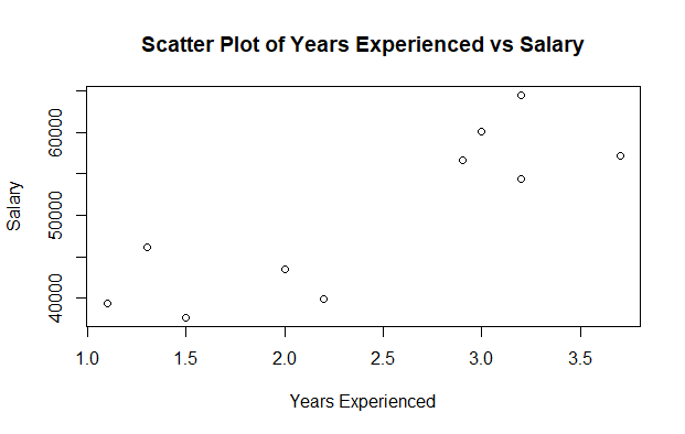
Linear Regression in R

Now, we have to find a line that fits the above scatter plot through which we can predict any value of y or response for any value of x 
The line which best fits is called the Regression line.

The equation of the regression line is given by: 

y = a + bx  

Where y is the predicted response value, a is the y-intercept, x is the feature value and b is the slope.
To create the model, let’s evaluate the values of regression coefficients a and b. And as soon as the estimation of these coefficients is done, the response model can be predicted. Here we are going to use the Least Square Technique.

The principle of least squares is one of the popular methods for finding a curve fitting a given data. Say be n observations from an experiment. We are interested in finding a curve 

Closely fitting the given data of size ‘n’. Now at x=x1 while the observed value of y is y1 the expected value of y from curve (1) is f(x1). Then the residual can be defined by… 

Similarly, residuals for x2, x3…xn are given by …

While evaluating the residual we will find that some residuals are positives and some are negatives. We are looking forward to finding the curve fitting the given data such that residual at any xi is minimum. Since some of the residuals are positive and others are negative and as we would like to give equal importance to all the residuals it is desirable to consider the sum of the squares of these residuals. Thus we consider:

and find the best representative curve.

Least Square Fit of a Straight Line 

Suppose, given a dataset of n observation from an experiment. And we are interested in fitting a straight line. 

to the given data.
Now consider: 

Now consider the sum of the squares of ei

Note: E is a function of parameters a and b and we need to find a and b such that E is minimum and the necessary condition for E to be minimum is as follows:

This condition yields: 

The above two equations are called normal equations which are solved to get the value of a and b.
The Expression for E can be rewritten as: 

The basic syntax for regression analysis in R is 

lm(Y ~ model) 

where Y is the object containing the dependent variable to be predicted and the model is the formula for the chosen mathematical model.
The command lm( ) provides the model’s coefficients but no further statistical information.

The following R code is used to implement Simple Linear Regression: 

R

install.packages('caTools')
library(caTools)
split = sample.split(data$Salary, SplitRatio = 0.7)
trainingset = subset(data, split == TRUE)
testset = subset(data, split == FALSE)

# Fitting Simple Linear Regression to the Training set
lm.r= lm(formula = Salary ~ Years_Exp,
         data = trainingset)
#Summary of the model
summary(lm.r)

Output:

Call:
lm(formula = Salary ~ Years_Exp, data = trainingset)
Residuals:
      1       2       3       5       6       8      10 
  463.1  5879.1 -4041.0 -6942.0  4748.0   381.9  -489.1 
Coefficients:
            Estimate Std. Error t value Pr(>|t|)   
(Intercept)    30927       4877   6.341  0.00144 **
Years_Exp       7230       1983   3.645  0.01482 * 
---
Signif. codes:  0 ‘***’ 0.001 ‘**’ 0.01 ‘*’ 0.05 ‘.’ 0.1 ‘ ’ 1
Residual standard error: 4944 on 5 degrees of freedom
Multiple R-squared:  0.7266,    Adjusted R-squared:  0.6719 
F-statistic: 13.29 on 1 and 5 DF,  p-value: 0.01482

Call: Using the “lm” function, we will be performing a regression analysis of “Salary” against “Years_Exp” according to the formula displayed on this line.

• Residuals: Each residual in the “Residuals” section denotes the difference between the actual salaries and predicted values. These values are unique to each observation in the data set. For instance, observation 1 has a residual of 463.1.
• Coefficients: Linear regression coefficients are revealed within the contents of this section.
• (Intercept): The estimated salary when Years_Exp is zero is 30927, which represents the intercept for this case.
• Years_Exp: For every year of experience gained, the expected salary is estimated to increase by 7230 units according to the coefficient for “Years_Exp”. This coefficient value suggests that each year of experience has a significant impact on the estimated salary.
• Estimate:The model’s estimated coefficients can be found in this column.
• Std. Error: “More precise estimates” can be deduced from smaller standard errors that are a gauge of the ambiguity that comes along with coefficient estimates.
• t value: The coefficient estimate’s standard error distance from zero is measured by the t-value. Its purpose is to examine the likelihood of the coefficient being zero by testing the null hypothesis. A higher t-value’s absolute value indicates a higher possibility of statistical significance pertaining to the coefficient.
• Pr(>|t|): This column provides the p-value associated with the t-value. The p-value indicates the probability of observing the t-statistic (or more extreme) under the null hypothesis that the coefficient is zero. In this case, the p-value for the intercept is 0.00144, and for “Years_Exp,” it is 0.01482.
• Signif. codes: These codes indicate the level of significance of the coefficients.
• Residual standard error: This is a measure of the variability of the residuals. In this case, it’s 4944, which represents the typical difference between the actual salaries and the predicted salaries.
• Multiple R-squared: R-squared (R²) is a measure of the goodness of fit of the model. It represents the proportion of the variance in the dependent variable that is explained by the independent variable(s). In this case, the R-squared is 0.7266, which means that approximately 72.66% of the variation in salaries can be explained by years of experience.
• Adjusted R-squared: The adjusted R-squared adjusts the R-squared value based on the number of predictors in the model. It accounts for the complexity of the model. In this case, the adjusted R-squared is 0.6719.
• F-statistic: The F-statistic is used to test the overall significance of the model. In this case, the F-statistic is 13.29 with 1 and 5 degrees of freedom, and the associated p-value is 0.01482. This p-value suggests that the model as a whole is statistically significant.

In summary, this linear regression analysis suggests that there is a significant relationship between years of experience (Years_Exp) and salary (Salary). The model explains approximately 72.66% of the variance in salaries, and both the intercept and the coefficient for “Years_Exp” are statistically significant at the 0.01 and 0.05 significance levels, respectively.

Predict values using predict function

R

# Create a data frame with new input values
new_data <- data.frame(Years_Exp = c(4.0, 4.5, 5.0))

# Predict using the linear regression model
predicted_salaries <- predict(lm.r, newdata = new_data)

# Display the predicted salaries
print(predicted_salaries)

Output:

       1        2        3 
65673.14 70227.40 74781.66 

Visualizing the Training set results: 

R

# Visualising the Training set results
ggplot() + geom_point(aes(x = trainingset$Years_Ex,
                          y = trainingset$Salary), colour = 'red') +
  geom_line(aes(x = trainingset$Years_Ex,
                y = predict(lm.r, newdata = trainingset)), colour = 'blue') +

  ggtitle('Salary vs Experience (Training set)') +
  xlab('Years of experience') +
  ylab('Salary')

Output:

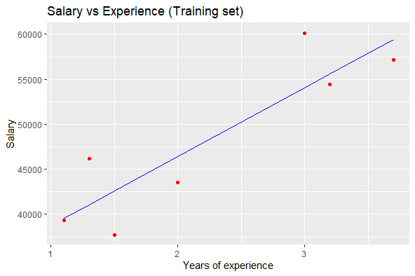
Training data visualization in Linear Regression in R

Visualizing the Testing set results:

R

# Visualising the Test set results
ggplot() +
  geom_point(aes(x = testset$Years_Exp, y = testset$Salary),
             colour = 'red') +
  geom_line(aes(x = trainingset$Years_Exp,
                y = predict(lm.r, newdata = trainingset)),
            colour = 'blue') +
  ggtitle('Salary vs Experience (Test set)') +
  xlab('Years of experience') +
  ylab('Salary')

Output:

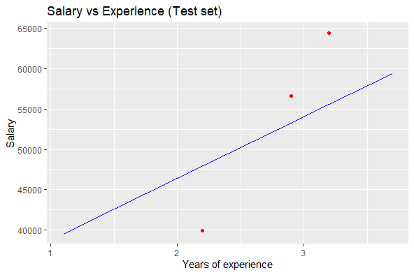
Testing Data Visualization in Linear Regression in R

Advantages of Simple Linear Regression in R:

1. Easy to implement: R provides built-in functions, such as lm(), to perform Simple Linear Regression quickly and efficiently.
2. Easy to interpret: Simple Linear Regression models are easy to interpret, as they model a linear relationship between two variables.
3. Useful for prediction: Simple Linear Regression can be used to make predictions about the dependent variable based on the independent variable.
4. Provides a measure of goodness of fit: Simple Linear Regression provides a measure of how well the model fits the data, such as the R-squared value.

Disadvantages of Simple Linear Regression in R:

1. Assumes linear relationship: Simple Linear Regression assumes a linear relationship between the variables, which may not be true in all cases.
2. Sensitive to outliers: Simple Linear Regression is sensitive to outliers, which can significantly affect the model coefficients and predictions.
3. Assumes independence of observations: Simple Linear Regression assumes that the observations are independent, which may not be true in some cases, such as time series data.
4. Cannot handle non-numeric data: Simple Linear Regression can only handle numeric data and cannot be used for categorical or non-numeric data.
5. Overall, Simple Linear Regression is a useful tool for modeling the relationship between two variables, but it has some limitations and assumptions that need to be carefully considered.