Signal Processing and Time Series (Data Analysis)

Signal processing is a field of engineering that focuses on analyzing analog and digital signals with respect to time. Time Series Analysis is one of the categories of signal processing. A time series is a sequence of data points recorded at regular intervals of time. Time series analysis is an important step before you develop a forecast of the series, and the order of the values is important in time series analysis. This process helps to extract meaningful statistics and other characteristics of data which helps to create an accurate forecast. Time series are widely used for data like weather, stock price, retail sales, etc… We will cover the following topics in this section:

1. Moving Average
2. Autoregressive Models
3. ARMA Models 

These are explained as following below. 1. Moving Average: A moving average (MA) is a widely used calculation to analyze time series. This specifies a window of data for a particular time period which is averaged each time by one period when new data is available. The two commonly used moving averages are:

1. Simple Moving Average (SMA) – SMA’s calculation provides the average data for a defined number of time periods. The mathematical formula as follows: Where, = parameter of the model n = total no of days
2. Exponential Moving Average (EMA) – Exponential moving average gives more priority to recent data. The mathematical formula as follows: Where, = current closing price = previous periods EMA [SMA for first calculation] k = 2 / (N+1) [exponential or smoothing constant] N = Total no of days considered for EMA calculation

EMA Calculation: Here we calculate EMA for 5 days. Normally for the first case either we take the current close price or previous 5 days SMA value to get the first EMA. For the below example, the current close price ($22.81) is taken as the first EMA value. The next step is to calculate the k value. Since the calculation is based on 5 days, N = 5 and k value is calculated as follows:

 k = 2/(5+1) = 0.3 

DAY	CLOSE PRICE	EMA	SMA
1	22.81	22.81	–
2	23.09	–	–

EMA for 2nd day is calculated as follows:

Current closing price = 23.09
Previous period EMA = 22.81
k = 0.3 

EMA 
= 22.81 + 0.3 * (23.09 - 22.81)
= 22.81 + 0.3 * 0.28
= 22.81 + 0.084
= 22.894 

DAY	CLOSE PRICE	EMA	SMA
1	22.81	22.81	–
2	23.09	22.89	–
3	22.91	–	–

EMA for 3rd day is calculated as follows:

Current closing price = 22.91
Previous period EMA = 22.89
k = 0.3 

EMA 
= 22.89 + 0.3 * (22.91 - 22.89)
= 22.89 + 0.3 * .02
= 22.89 + .006
= 22.896 

DAY	CLOSE PRICE	EMA	SMA
1	22.81	22.81	–
2	23.09	22.89	–
3	22.91	22.89	–

SMA Calculation: Since we considered total days (N) as 5, the SMA is calculated as the average of 5 latest close price.

DAY	CLOSE PRICE	EMA	SMA
1	22.81	22.81	–
2	23.09	22.89	–
3	22.91	22.89	–
4	23.23	22.99	–
5	22.83	22.94	–

SMA for 5 days is calculated as follows:

SMA 
= (22.81 + 23.09 + 22.91 + 23.23 + 22.83) / 5
= 114.87 / 5 
= 22.97  

DAY	CLOSE PRICE	EMA	SMA
1	22.81	22.81	–
2	23.09	22.89	–
3	22.91	22.89	–
4	23.23	22.99	–
5	22.83	22.94	22.97
6	23.05	–	–

2. Autoregressive Models: An autoregressive model can be used to predict future data based on past data. In this model, data is assumed to depend on its previous data. Since autoregressive models totally depend on past data to generate future models, there are chances of generating inaccurate data under certain conditions such as financial crises or sudden technological changes. The mathematical formula as follows: AR Calculation: The below data provide the stock price of today(t), one day before (t-1), two days before (t-2) and three days before (t-3).

t	t-1	t-2	t-3
23.23	22.91	23.09	22.81
22.83	23.23	22.91	23.09
23.05	22.83	23.23	22.91
23.02	23.05	22.83	23.23
23.29	23.02	23.05	22.83
23.41	23.29	23.02	23.05
23.49	23.41	23.29	23.02
24.6	23.49	23.41	23.29
24.63	24.6	23.49	23.41
24.51	24.63	24.6	23.49
23.73	24.51	24.63	24.6
23.31	23.73	24.51	24.63
23.53	23.31	23.73	24.51
23.06	23.53	23.31	23.73
23.25	23.06	23.53	23.31
23.12	23.25	23.06	23.53
22.8	23.12	23.25	23.06
22.84	22.8	23.12	23.25

With the above stock price data, you need to perform the linear regression to get the parameters required for AR model. For this, you can use data analysis feature from excel. For regression, you can provide t data as Y input and (t-1), (t-2), (t-3) as X input. Microsoft excel will provide you the below result. Regression Statistics:

Multiple R: 0.786903932
R Square: 0.619217798
Adjusted R Square: 0.537621612
Standard Error: 0.398415364
Observations: 18 

	Coefficients	Standard Error
Intercept	8.59250239	4.494566177
t-1	0.840795074	0.249566271
t-2	0.100511124	0.331626753
t-3	-0.308260596	0.250400704

Let’s look into how to use the output values from regression. Previous Stock Data:

Coefficient of t-1 = 0.840795074 and Close price = 22.8
Coefficient of t-2 = 0.100511124 and Close price = 23.12
Coefficient of t-3 = -0.308260596 and Close price = 23.25 

Value of Constant:

Coefficient of Intercept = 8.59250239 = 8.6 

Standard Error:

t-1 = 0.249566271
t-2 = 0.331626753
t-3 = -0.250400704 

Standard Error 
= 0.25 + 0.33 - 0.25
= 0.33 

AR 
= 8.6 + [ (0.84*22.8) + (0.1*23.12) + (-0.31*23.25) ] + 0.33
= 8.6 + [ 19.15 + 2.31 - 7.20] + 0.33
= 8.6 + 14.26 + 0.33
= 23.19 

Rather than going through the entire calculation, you can predict tomorrow stock price with today stock price and R square value (refer regression statistics output above). Suppose that, the stock price of today is $22.84, then tomorrow’s stock price is calculated as:

AR(t+1) = Coefficient of Intercept + (R square * Today's Price) 
                                        + Standard Error

R Square = 0.619217798 

Standard Error (from regression statistics) = 0.398415364 

AR 
= 8.6 + (0.619*22.84) + 0.39
= 8.6 + 14.14 + 0.39
= 23.13 

3. ARMA Models: ARMA model is another tool used to forecast a time series. These models are based on the combination of both autoregressive and moving average models. In the AR model, we use past data for regressing the variable and in the MA model, we use the sum of the mean of the time series for a forecast. Since the ARMA model is the combination of both AR part and MA part, this model is referred to as ARMA(p, q) model where p is the AR part and q is the MA part. 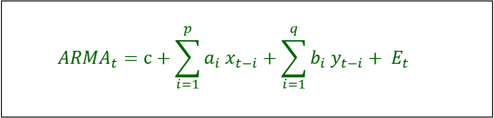The mathematical formula is as follows: Where, = the autoregressive model’s parameter = the moving average model’s parameter c = a constant = error term’s [White Noise]