Separating Hyperplanes in SVM

Support Vector Machine is the supervised machine learning algorithm, that is used in both classification and regression of models. The idea behind it is simple to just find a plane or a boundary that separates the data between two classes.

Support Vectors:

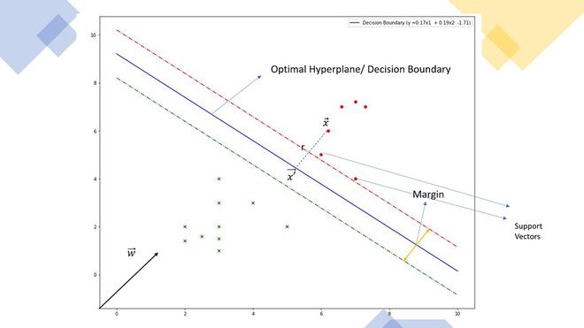
Support vectors are the data points that are close to the decision boundary, they are the data points most difficult to classify, they hold the key for SVM to be optimal decision surface. The optimal hyperplane comes from the function class with the lowest capacity i.e minimum number of independent features/parameters.

Separating Hyperplanes:

Below is an example of a scatter plot:

In the above scatter, Can we find a line that can separate two categories. Such a line is called separating hyperplane. So, why it is called a hyperplane, because in 2-dimension, it’s a line but for 1-dimension it can be a point, for 3-dimension it is a plane, and for 3 or more dimensions it is a hyperplane

Now, we understand the hyperplane, we also need to find the most optimized hyperplane. The idea behind that this hyperplane should farthest from the support vectors. This distance b/w separating hyperplanes and support vector known as margin. Thus, the best hyperplane will be whose margin is the maximum.

Generally, the margin can be taken as 2*p, where p is the distance b/w separating hyperplane and nearest support vector. Below is the method to calculate linearly separable hyperplane. 

A separating hyperplane can be defined by two terms: an intercept term called b and a decision hyperplane normal vector called w. These are commonly referred to as the weight vector in machine learning. Here b is used to select the hyperplane i.e perpendicular to the normal vector. Now since all the plane x in the hyperplane should satisfy the following equation:

Now, consider the training D such that where  represents the n-dimesnsional data point and class label respectively. The value of class label here can be only either be -1 or +1 (for 2-class problem). The linear classifier is then:

However, the functional margin is by definition of above is unconstraint, so we need to formulize the distance b/w a data point x and the decision boundary. The shortest distance b/w them is of course the perpendicular distance i.e parallel to the normal vector . A unitary vector in the direction of this normal vector is given by. Now, 

 can be defined as: 

Replace x’ by x in the linear classifier equation gives: 

Now, solving for r gives following equation: 

where, r is the margin. Now, since the 

. The distance equation for a data point to hyperplane for all items in the data could be written as: 

or, the above equation for each data point: 

Here, the geometric margin is: 

We need to maximize the geometric margin such that: 

Maximizing  is same as minimizing the that is, we need to find w and b such that: 

 is minimum 

Here, we are optimizing a quadratic equation with linear constraint. Now, this leads us to find the solution dual problems.  

Duality Problem:

In optimization, the duality principle states that optimization problems can either be viewed from a different perspective: the primal problem and the dual problem The solution to the dual problem provides a lower bound to the solution of the primal (minimization) problem.

An optimization problem can be typically written as:

where, f is objective function g and h are constraint function. The above problem can be solved by a technique such as Lagrange multipliers. 

Lagrange multipliers

Lagrange multiplier is a way of finding local minima and maxima for the functions with an equality constraint. Lagrange multipliers can be described for the 

In Lagrangian equation: 

Suppose, we define the function such that 

The above function is known as Lagrangian, now, we need to find  is 0 i.e point where gradient of functions f and g are parallel. 

Example

Consider having three points with points (1,2) and (2,0) belonging to one class and (3,2) belonging to another, geometrically, we can observe that the maximum margin line will be parallel to line connecting points of the two classes. (1,1) and (2,3) given a weight vector as (1,2). The optimal decision surface (separating hyperplane) will intersect at (1.5,2). Now, we can calculate bias using this conclusion: 

.Now, the decision surface equation becomes: 

Now, since sign , to minimize the , we need to check for the equality constraint or the support vectors. Let’s take w=(a, 2a) for some a such that: 

Solving above equation gives: 

this means the margin becomes: 

Implementation

In this implementation, we will verify the above example using the sklearn library and tried to model the above example: 

Python3

# Import Necessary libraries/functions
import numpy as np
import matplotlib.pyplot as plt
from sklearn.svm import SVC

# define the dataset
X = np.array([[1,1],
             [2,0],
             [2,3]])
Y = np.array([0,0,1])

# define support vector classifier with linear kernel

clf = SVC(gamma='auto', kernel ='linear')

# fit the above data in SVC
clf.fit(X,Y)

# plot the decision boundary ,data points,support vector etcv
w = clf.coef_[0]
a = -w[0] / w[1]

xx = np.linspace(0,12)
yy = a * xx - clf.intercept_[0] / w[1]
y_neg = a * xx - clf.intercept_[0] / w[1] + 1
y_pos = a * xx - clf.intercept_[0] / w[1] - 1
plt.figure(1,figsize= (15, 10))
plt.plot(xx, yy, 'k',
         label=f"Decision Boundary (y ={w[0]}x1  + {w[1]}x2  {clf.intercept_[0] })")
plt.plot(xx, y_neg, 'b-.',
         label=f"Neg Decision Boundary (-1 ={w[0]}x1  + {w[1]}x2  {clf.intercept_[0] })")
plt.plot(xx, y_pos, 'r-.',
         label=f"Pos Decision Boundary (1 ={w[0]}x1  + {w[1]}x2  {clf.intercept_[0] })")

for i in range(3):
  if (Y[i]==0):
      plt.scatter(X[i][0], X[i][1],color='red', marker='o', label='negative')
  else:
      plt.scatter(X[i][0], X[i][1],color='green', marker='x', label='positive')
plt.legend()
plt.show()

# calculate margin
print(f'Margin : {2.0 /np.sqrt(np.sum(clf.coef_ ** 2)) }')

Margin : 2.236

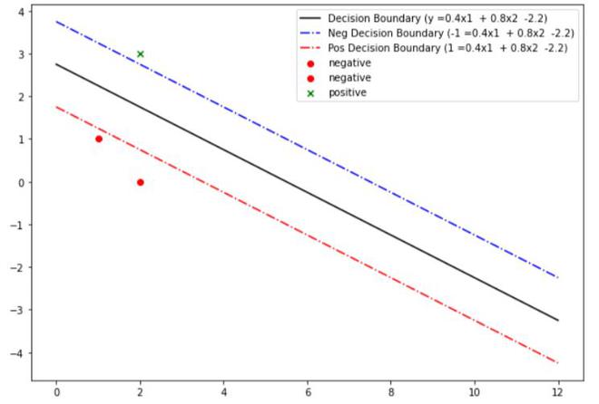
FInal SVM decision boundary

References:

• Stanford NLP