SciPy – Integration of a Differential Equation for Curve Fit

In Machine Learning, often what we do is gather data, visualize it, then fit a curve in the graph and then predict certain parameters based on the curve fit. If we have some theoretical data we can use curve fitting from the verified dataset to extract the equation and verify it. So to find the equation of a curve of any order be it linear, quadratic or polynomial, we use Differential Equations and then integrating that equation we can get the curve fit.
In Python SciPy, this process can be done easily for solving the differential equation by mathematically integrating it using odeint(). The odeint(model, y0, t) can be used to solve any order differential equation by taking three or more parameters. 

Parameters : 
model– the differential equation  
y0– Initial value of Y 
t– the time space for which we want the curve(basically the range of x) 

Let’s illustrate this with an example: 

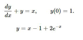
Code: To solve the equation to get y = x – 1 + 2 (e^-x) as the solution 

python3

import numpy as np
from scipy.integrate import odeint
import matplotlib.pyplot as plt

from scipy.integrate import odeint

# Define a function which calculates the derivative by making dy/dx as
# the subject of formula in the given above equation
def dy_dx(y, x):
    return x - y

#Here we define the graph limits for x
xs = np.linspace(-5,5,100)

#Initially y=1 given
y0 = 1.0

# This scipy.integrate.odeint() integrates the given equation by taking
# 3 parameters odeint(model,y0,t)
# model- the differential equation function
# y0-the initial value of y
# t- the timepoints for which we need to plot the curve
ys = odeint(dy_dx, y0, xs)
ys = np.array(ys).flatten()

# By using the matplotlib.pyplot library we plot the curve after integration
plt.rcParams.update({'font.size': 14})  # increase the font size
plt.xlabel("x-values")
plt.ylabel("Y- values")
plt.title('Curve of -> y=x-1+2*(e^-x)')
plt.plot(xs, ys,color='green')

Output:
This is the graph generated by using the scipy.integrate.odeint( ) which can be seen below and further be used for curve fitting – for analyzing the data in Machine learning. 

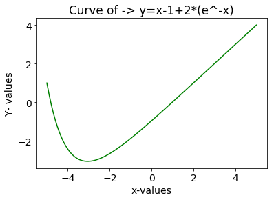
The Graph generated after integrating the differential equation