Excel ROWS and COLUMNS Functions with Examples

In Microsoft Excel, where precision and efficiency reign supreme, mastering the art of maneuvering through cells and worksheets is indispensable. Two indispensable components in your Excel toolbox are the ROW and COLUMN functions, each meticulously crafted to execute discrete functions that can substantially facilitate your data analysis and manipulation endeavors. Within the confines of this article, we shall delve into the multifaceted capabilities of these functions and elucidate how they can seamlessly optimize your spreadsheet tasks. Whether you possess the seasoned prowess of an Excel virtuoso or are just embarking on your spreadsheet odyssey, comprehending the intrinsic attributes of the ROW and COLUMN functions represents an elemental stride in your journey toward Excel proficiency.

What is Excel ROWS and COLUMNS Functions

Excel’s Rows and Columns are like the building blocks of your spreadsheet. Think of columns as the vertical parts, and rows as the horizontal ones. Each cell, range of cells, or table in Excel is made up of these rows and columns. In simpler terms, when you look from top to bottom in Excel, you’re looking at columns. When you look from left to right, you’re looking at rows. To give you an idea of the vastness, there are 16,384 columns and 1,048,576 rows in a single Excel worksheet. It’s like a huge grid where you can place your data.

What is a Row in Excel

A row consists of cells arranged horizontally, and each row is uniquely identified by a number. In Excel, columns are labeled alphabetically, starting with A for the leftmost column.

What is a Column in Excel

A column is formed by cells stacked vertically, and each column is designated by a specific letter. The topmost row in Excel is numbered as 1, the row below it as 2, and so forth.

What is a Cell in Excel

A cell is created at the intersection of a row and a column. In Excel, cells are referred to by their column letter followed by the row number. For example, the cell at the top left corner is denoted as A1.

What is the difference between ROW and ROWS functions in Excel?

ROW Function: This particular function serves the purpose of extracting the precise row number linked to a designated cell or range. It can be applied with an optional reference argument that specifies the cell or range for which you intend to procure the row number.

For example, Employ the formula “=ROW(A54),” it will discreetly furnish the row number of cell A53, which discreetly stands at 53.

ROWS Function: The ROWS function discreetly undertakes the task of enumerating the rows nestled within a given range of cells. It simply demands a single argument – the range over which you clandestinely wish to compute the row count.

For instance, the formula “=ROWS(A10:A53)” will skillfully yield the tally of rows within the covertly specified range A10:A53, which slyly amounts to 43.

In conclusion, the ROW function adroitly targets the row number of a covertly chosen cell, while the ROWS function surreptitiously quantifies the rows existing within a selected cell range.

ROWS and COLUMNS Functions in Excel

It provides a numerical output, or in the case of multi-cell array formulas, a sequence of successive numbers. This functionality proves useful because it allows for the creation of formulas that need to be replicated vertically, horizontally, or in both directions in an efficient manner.

What is ROWS Function in Excel

The ROW Function has several Purposes:

Row Number for a Cell Reference: It returns the row number associated with a specified cell reference.

Current Row Number: It provides the row number of the cell where the function is placed within the worksheet.

Multiple Row Numbers: When used in an array formula, it can generate a series of row numbers corresponding to its locations.

What is COLUMN Functions in Excel

The COLUMN Function can be used for the following things:

Current Column Number: It furnishes the column number of the cell where the function is positioned within the worksheet.

Column Number for a Cell Reference: It returns the column number for a given cell reference.

In an Excel worksheet, rows are sequentially numbered from top to bottom, with the first row assigned number 1. Columns are numbered from left to right, starting with column A as the initial column.

Consequently, if applied, the ROW function would yield 1 for the first row, and for the final row, it would return the value, 1.048,576, which is the total number of rows available in an Excel worksheet.

How to Use ROW Function in Excel

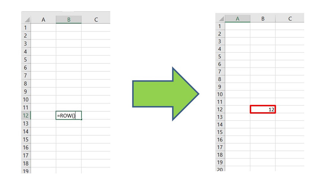
The ROW( ) function basically returns the row number for reference. 

Syntax:

=ROW([reference])

ROW Function Example

=ROW(G100); Returns 100 as output
as G100 is in the 100th row in the Excel sheet

If we write no argument inside the ROW( ) it will return the row number of the cell in which we have written the formula.

Here the following returns are achieved:

=ROW(A67) // Returns 67
=ROW(B4:H7) // Returns 4

What is ROWS Function

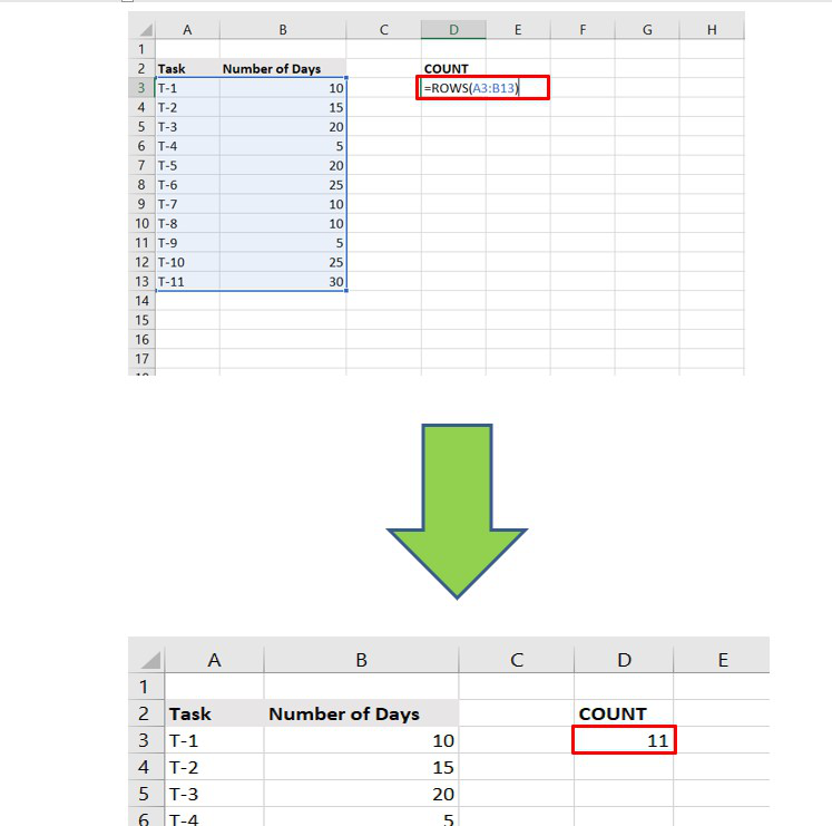
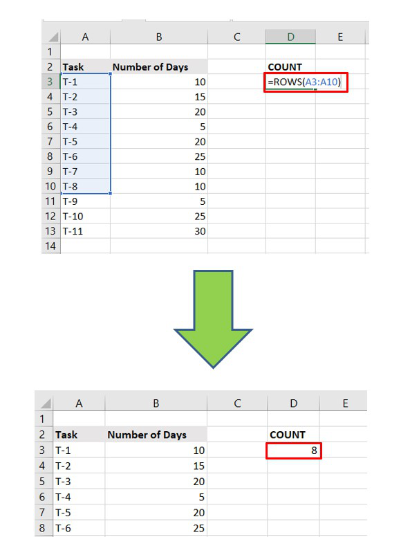
It is the extended version of the ROW function. ROWS function is used to return the number of rows in a cell range.

Syntax:

=ROWS([array])

How to use the ROWS formula in Excel

=ROWS(A2:A11) // Returns 10 as there are ten rows

It is important to note that writing the column name is trivial here. We can also write :

=ROWS(2:13) // Returns 12

What is COLUMN Function in Excel

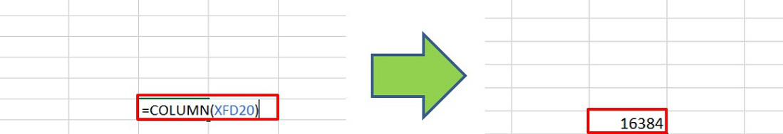
The column function usually returns the column number of a reference. There are 16,384 columns in Excel from the 2007 version. It returns the value 1 to 16,384.

Syntax:

=COLUMN([reference])

COLUMN Function Example

=COLUMN(E20) // Returns 5 as output
as E is the fifth column in the Excel sheet

Last Column of Excel

Similar to the ROW function, the argument is not mandatory. If we don’t write any argument, it will return the index of the column in which the formula is written.

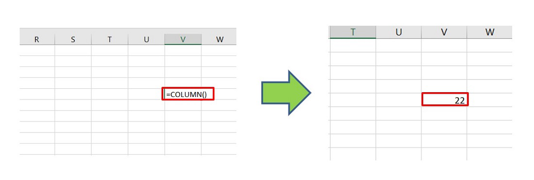
What is COLUMNS Function in Excel

It is the extended version of the COLUMN( ). It returns the number of columns for a given cell range.

Syntax:

=COLUMNS([array])

COLUMNS Function Example

=COLUMNS(B12:E12) // Returns 4 as output as
there are 4 columns in the given range

It is important to note that writing the row number is trivial here. We can also write :

=COLUMNS(B:E) // Returns 4

ROWS And COLUMNS Functions in Array Formulas

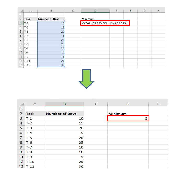
We can use the ROWS( ) and COLUMNS( ) in array formulas using SMALL( ), LARGE( ), VLOOKUP( ) functions in Excel.

Example : The smallest value is returned to the provided cell range.

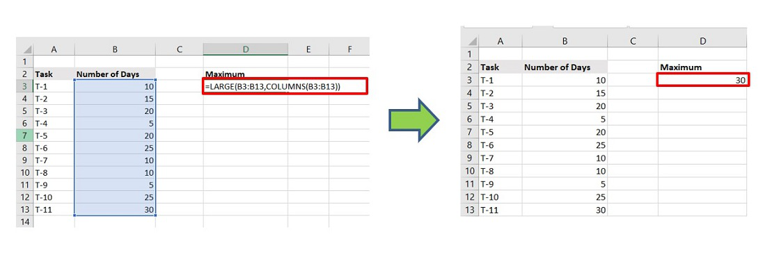
The largest value is returned to the provided cell range.

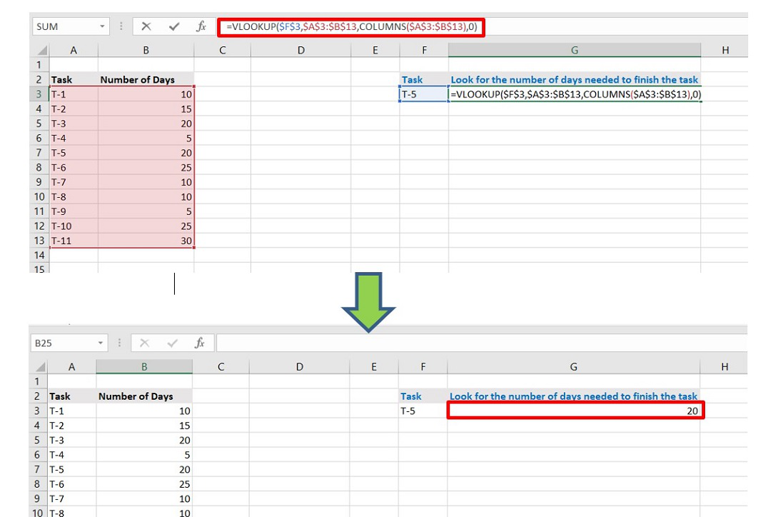
Say, we need to find the number of days needed to complete Task number 5. 

How to Use ROWS And COLUMNS Functions in Array Formulas

Step 1: Choose any cell and write the name of the Task

Step 2: Beside that cell write the Formula

=VLOOKUP($F$3,$A$3:$B$13,COLUMNS($A$3:$B$13),0)

F3 : Reference of the Task T-5

A3:B13 : Cell range of the entire table for VLOOKUP to search

Step 3: Press Enter

Now, it can be observed it returns 20 as output which is perfect as per the data set.

FAQs

What are the ROWS and COLUMNS Function in Excel?

The ROWS and COLUMNS Function in Excel are used to count the number of rows and columns in a specified range, respectively. ROWS counts the rows, while COLUMNS ocunts the columns.

How to use the ROWS Function to count rows in Excel?

The ROWS Function is used as follows: ‘=ROWS(range)’. For example ‘=ROWS(A1:A10) will count the number of rows in the range A1:A10.

How to use the ROW Function to get the row number of a specific cell?

The ROW function returns the row number of a given cell. For example : ‘=ROW(A2)’ will return the row number of cell A2.

What are the limitations of using ROWS and COLUMNS functions?

Remember that using functions on a very large ranges could impact performance . Also, be cautions when using these functions in complex array formulas, as they may increase calculation times.