Root Locus using MATLAB

In control systems, root locus analysis is a graphical strategy for looking at how the foundations of a system change with variety of a specific system boundary, generally an addition inside a feedback system.

Purpose of root locus in control system are as follows:

1. To find the stability
2. To check a point is on root locus or not
3. To find system gain i.e. “k” or system parameter

Construction rules of a root locus :

Rule 1: A point will exists on real axis, root locus branches if the sum of poles and zeros to the right hand side of the point must be odd.

Rule 2: Asymptotes: They are root locus branches which starts on real axis and approaches to infinity.

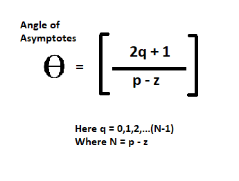
Number of asymptotes “N = P – Z”

Here “P” is number of poles and “Z” is number of zeros

Rule 3: Angle of Asymptotes

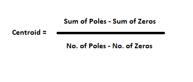
Rule 4: Centroid : Meeting point of asymptotes on real axis is called as centroid

Rule 5: Break Point (BP): There are two types

1. Break Away Point (BAP)
2. Break In Point (BIP)

Rule 6: Root locus intersection point (IP) with imaginary axis.

Rule 7: 

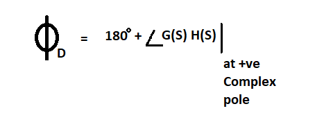
a) Angle of departure: It is calculated for complex conjugated poles or imaginary poles

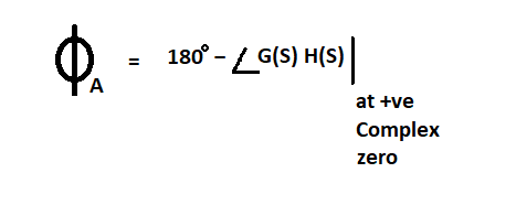
b) Angle of  arrival: It is calculated for complex conjugate zeros or imaginary zeros

Code :

% Row of 1×2
NUM = [1 10];

% Row of 1×4
DEN = [1 6 8 0];

% Row of 1×2
poly1 = [1 2];

% Row of 1×2
poly2 = [1 4];

% convolves vectors poly1 and poly2,
% multiplying the polynomials whose coefficients
% are the elements of poly1 and poly2
poly = conv(poly1, poly2);

% returns the roots of the polynomial
% represented by DEN as a column vector
roots(DEN);

% Continuous time transfer function
sys = tf(NUM, DEN);

% GUI for per-forming Root Locus analysis
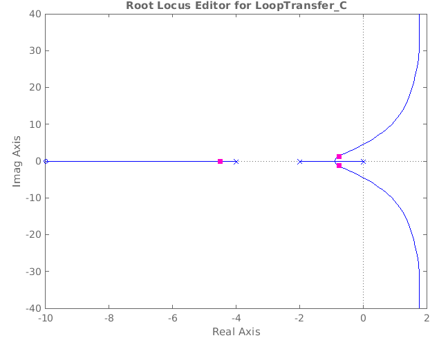
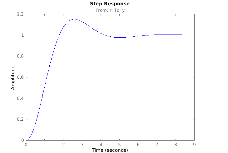
rltool(sys);

Output :