Robust Correlation

Last Updated : 19 Mar, 2024

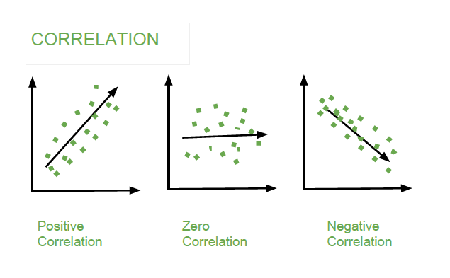
Correlation is a statistical tool that is used to analyze and measure the degree of relationship or degree of association between two or more variables. There are generally three types of correlation:

Positive correlation: When we increase the value of one variable, the value of another variable increased respectively, this is called Positive Correlation.
Negative correlation: When we increase the value of one variable, the value of another variable decreases respectively, this is called negative Correlation.
Zero correlation: When the change in the value of one variable does not impact another substantially, then it is called zero correlation.

Pearson Correlation:

Pearson correlation is the most common way of calculating the correlation. It is denoted by r. Consider for two variables x and y, it is represented by the following formula:

$r = \frac{\sum_{i=1}^{n} (x_i - \overline{x})(y_i - \overline{y})} {\sqrt{\sum_{i=1}^{n} (x_i - \overline{x})^2(y_i - \overline{y})^2}}$

A value closer to -1 represents a perfectly negative correlation, whereas 0 represents no correlation and 1 represents a strong positive correlation.

The Pearson correlation coefficient is a good estimator of correlation between two variables for normal distribution. However, it does not fill the criteria of the robust estimator because it is not:

Resistant: This means changing a small fraction of data even by a huge amount does not considerably affect the value of the estimate.
Robustness of Efficiency: the statistic has high efficiency in a variety of situations rather than in any one situation. Efficiency means that the estimate is close to the optimal estimate given that we know what distribution that the data comes from.

Efficiency can be measure using the following formula:

$Efficiency = \frac{lowest-variance-possible}{actual-variance}$

Percentage Bend Correlation:

Percent bend correlation was proposed by shoemaker and Hettmanspergr in 1982 and also mentioned by Wilcox in his book. This correlation is both resistant and robust to efficiency.

Following are the steps to perform Percentage Bend correlation on two variables X and Y:

Set m = (1-\beta) *m + 0.5, Round m to nearest integer. Here, \beta is between 0 and 0.5
Take W_{i} = |X_{i} – M_{x}| for i = 1, 2, …n, where M_x is the median of X.
Sort W_i in the ascending order.
$\hat{W_x} = W(m)$ , where W(m) is the estimate of the (1-\beta) quantile of W.
Sort the X values.
Computer the number of values \frac{(X_{i} – M_{x})}{\hat{W}_{x}(\beta)} that are <-1 and store in i_1 and the number that are > +1 and store in $i_2$ respectively. Then compute the following:

$S_{x} = \sum_{i=i1+1}^{n-i2}{X_{i}}$

$\hat{\phi}_{x} = \frac{\hat{W}_{x}(i2 - i1) + S_{x}}{n - i1 - i2}$

$U_{i} = \frac{X_{i} - \hat{\phi}_{x}}{\hat{W}_{x}}$

Repeat the above steps for the Y estimator to get \hat{W_y}, \hat{\phi}_{y} and V_i.
Define the function:

$\Psi(x) = \max[-1, \min(1,x)]$

therefore compute,

$A_i = \Psi (U_i), B_i = \Psi (V_i)$

Calculate the percent bend correlation:

$\rho_{pb} = \frac{\sum_{i=1}^{n}{A_{i}B_{i}}} {\sqrt{\sum_{i=1}^{n}{A_{i}^2}\sum_{i=1}^{n}{B_{i}^2}}}$

Winsorized Correlation:

The standard correlation like Pearson is sometimes heavily influenced by extreme values. The Winsorized correlation solves this by setting the tail values equal to a certain percentile value.

For example, for a 90% Winsorized correlation, the bottom 5% of the values are set equal to the value corresponding to the 5th percentile while the upper 5% of the values are set equal to the value corresponding to the 95th percentile. Then the standard correlation is applied.

Implementation:

In this implementation, we will be using the motor trend car Road Tests dataset available in the graphics library in R. It is very popular and easily available. This dataset contains 32 observations of 11 different variables related to cars. We will be performing the correlation analysis between these variables (Pearson, percentage bend and winsorized) and plot them.

# Install the required packages
install.packages("dplyr")
install.packages("correlation")
install.packages("see")

# import required packages
library(dplyr)
library(correlation)
library(see)

# Load data
data("mtcars")
# check help for mtcars data
?mtcars

## Description
# The data was extracted from the 1974 Motor Trend US magazine, 
# and comprises fuel consumption and 10 aspects of automobile
# design and performance for 32 automobiles 
#(1973–74 models).
 
## Usage
# mtcars

## Format
# A data frame with 32 observations on 11 (numeric) variables.
# 
# [, 1]    mpg    Miles/(US) gallon
# [, 2]    cyl    Number of cylinders
# [, 3]    disp    Displacement (cu.in.)
# [, 4]    hp    Gross horsepower
# [, 5]    dart    Rear axle ratio
# [, 6]    wt    Weight (1000 lbs)
# [, 7]    qsec    1/4 mile time
# [, 8]    vs    Engine (0 = V-shaped, 1 = straight)
# [, 9]    am    Transmission (0 = automatic, 1 = manual)
# [,10]    gear    Number of forward gears
# [,11]    carb    Number of carburetors

## Source
# Henderson and Velleman (1981), Building multiple regression
# models interactively. Biometrics, 37, 391–411.

# perform different correlation and print summary

# pearson correlation
pearson_corr = correlation(mtcars)
pearson_summary = summary(pearson_corr)
print(pearson_summary)

# percentage bend correlation
pbc_corr = correlation(mtcars,method='percentage')
pbc_summary= summary(pbc_corr)
print(pbc_summary)

# winsorized correlation
wins_corr = correlation(mtcars, winsorize = 0.2)
winsor_summary = summary(wins_corr)
print(winsor_summary)

# plot different correlation analysis
pearson_summary%>%plot()
pbc_summary%>%plot()
winsor_summary%>%plot()

# Correlation Matrix (pearson-method)

Parameter |    carb |    gear |       am |       vs |     qsec |       wt |     dart |       hp |     disp |      cyl
---------------------------------------------------------------------------------------------------------------------
mpg       |  -0.55* |    0.48 |   0.60** |   0.66** |     0.42 | -0.87*** |  0.68*** | -0.78*** | -0.85*** | -0.85***
cyl       |   0.53* |   -0.49 |   -0.52* | -0.81*** |   -0.59* |  0.78*** | -0.70*** |  0.83*** |  0.90*** |         
disp      |    0.39 |  -0.56* |   -0.59* | -0.71*** |    -0.43 |  0.89*** | -0.71*** |  0.79*** |          |         
hp        | 0.75*** |   -0.13 |    -0.24 | -0.72*** | -0.71*** |   0.66** |    -0.45 |          |          |         
dart      |   -0.09 | 0.70*** |  0.71*** |     0.44 |     0.09 | -0.71*** |          |          |          |         
wt        |    0.43 |  -0.58* | -0.69*** |   -0.55* |    -0.17 |          |          |          |          |         
qsec      | -0.66** |   -0.21 |    -0.23 |  0.74*** |          |          |          |          |          |         
vs        |  -0.57* |    0.21 |     0.17 |          |          |          |          |          |          |         
am        |    0.06 | 0.79*** |          |          |          |          |          |          |          |         
gear      |    0.27 |         |          |          |          |          |          |          |          |         

p-value adjustment method: Holm (1979)>

# Correlation Matrix (percentage-method)

Parameter |     carb |    gear |       am |       vs |     qsec |       wt |     dart |       hp |     disp |      cyl
----------------------------------------------------------------------------------------------------------------------
mpg       |  -0.64** |   0.55* |   0.58** |  0.68*** |     0.48 | -0.90*** |  0.68*** | -0.90*** | -0.88*** | -0.91***
cyl       |    0.58* |  -0.55* |   -0.52* | -0.81*** |  -0.60** |  0.85*** | -0.72*** |  0.91*** |  0.94*** |         
disp      |     0.47 | -0.61** |  -0.60** | -0.73*** |    -0.50 |  0.88*** | -0.74*** |  0.89*** |          |         
hp        |  0.70*** |   -0.37 |    -0.40 | -0.79*** | -0.69*** |  0.80*** |  -0.59** |          |          |         
dart      |    -0.11 | 0.78*** |  0.73*** |     0.47 |     0.13 | -0.76*** |          |          |          |         
wt        |    0.53* | -0.64** | -0.76*** |   -0.57* |    -0.26 |          |          |          |          |         
qsec      | -0.68*** |   -0.13 |    -0.17 |  0.80*** |          |          |          |          |          |         
vs        |  -0.62** |    0.27 |     0.17 |          |          |          |          |          |          |         
am        |    -0.07 | 0.80*** |          |          |          |          |          |          |          |         
gear      |     0.11 |         |          |          |          |          |          |          |          |         

p-value adjustment method: Holm (1979)>

# Winsorized Correlation Matrix

Parameter |    carb |     gear |       am |       vs |    qsec |       wt |     dart |       hp |     disp |      cyl
---------------------------------------------------------------------------------------------------------------------
mpg       | -0.63** |   0.65** |    0.55* |  0.70*** |    0.49 | -0.86*** |  0.67*** | -0.88*** | -0.87*** | -0.93***
cyl       |  0.60** | -0.68*** |   -0.52* | -0.81*** | -0.60** |  0.87*** | -0.74*** |  0.90*** |  0.94*** |         
disp      |    0.45 | -0.74*** |   -0.57* | -0.72*** |  -0.51* |  0.85*** | -0.74*** |  0.89*** |          |         
hp        | 0.69*** |   -0.56* |    -0.37 | -0.79*** | -0.63** |  0.77*** |  -0.60** |          |          |         
dart      |   -0.12 |  0.88*** |  0.72*** |    0.50* |    0.22 | -0.76*** |          |          |          |         
wt        |   0.53* | -0.69*** | -0.78*** |   -0.56* |   -0.29 |          |          |          |          |         
qsec      | -0.61** |     0.15 |    -0.12 |  0.84*** |         |          |          |          |          |         
vs        | -0.62** |     0.45 |     0.17 |          |         |          |          |          |          |         
am        |   -0.11 |  0.78*** |          |          |         |          |          |          |          |         
gear      |   -0.03 |          |          |          |         |          |          |          |          |         

p-value adjustment method: Holm (1979)