Regression Analysis in R Programming

In statistics, Logistic Regression is a model that takes response variables (dependent variable) and features (independent variables) to determine the estimated probability of an event. A logistic model is used when the response variable has categorical values such as 0 or 1. For example, a student will pass/fail, a mail is a spam or not, determining the images, etc. In this article, we’ll discuss regression analysis, types of regression, and implementation of logistic regression in R programming.

Regression Analysis in R

Regression analysis is a group of statistical processes used in R programming and statistics to determine the relationship between dataset variables. Generally, regression analysis is used to determine the relationship between the dependent and independent variables of the dataset. Regression analysis helps to understand how dependent variables change when one of the independent variables changes and other independent variables are kept constant. This helps in building a regression model and further, helps in forecasting the values with respect to a change in one of the independent variables. On the basis of types of dependent variables, a number of independent variables, and the shape of the regression line, there are 4 types of regression analysis techniques i.e., Linear Regression, Logistic Regression, Multinomial Logistic Regression, and Ordinal Logistic Regression.

Types of Regression Analysis

Linear Regression

Linear Regression is one of the most widely used regression techniques to model the relationship between two variables. It uses a linear relationship to model the regression line. There are 2 variables used in the linear relationship equation i.e., predictor variable and the response variable.

y = ax + b

where, 

• y is the response variable
• x is the predictor variable
• a and b are the coefficients

The regression line created using this technique is a straight line. The response variable is derived from predictor variables. Predictor variables are estimated using some statistical experiments. Linear regression is widely used but these techniques is not capable of predicting the probability.

Logistic Regression

On the other hand, logistic regression has an advantage over linear regression as it is capable of predicting the values within the range. Logistic regression is used to predict the values within the categorical range. For example, male or female, winner or loser, etc.

Logistic regression uses the following sigmoidal function:

where, 

• y represents response variable
• z represents equation of independent variables or features

Multinomial Logistic Regression

Multinomial logistic regression is an advanced technique of logistic regression that takes more than 2 categorical variables unlike, in logistic regression which takes 2 categorical variables. For example, a biology researcher found a new type of species and the type of species can be determined by many factors such as size, shape, eye color, the environmental factor of its living, etc.

Ordinal Logistic Regression

Ordinal logistic regression is also an extension of logistic regression. It is used to predict the values as different levels of category (ordered). In simple words, it predicts the rank. For example, a survey of the taste quality of food is created by a restaurant, and using ordinal logistic regression, a survey response variable can be created on a scale of any interval such as 1-10 which helps in determining the customer’s response to their food items.

Implementation of Logistic Regression in R programming

In R language, a logistic regression model is created using glm() function. 

Syntax:glm(formula, family = binomial)
Parameters:
formula: represents an equation on the basis of which model has to be fitted. 
family: represents the type of function to be used i.e., binomial for logistic regression 

To know about more optional parameters of glm() function, use below command in R: 

help("glm")

Example:

Let us assume a vector of IQ level of students in a class. Another vector contains the result of the corresponding student i.e., fail or pass (0 or 1) in an exam. 

r

# Generate random IQ values with mean = 30 and sd =2
IQ <- rnorm(40, 30, 2)

# Sorting IQ level in ascending order
IQ <- sort(IQ)

# Generate vector with pass and fail values of 40 students
result <- c(0, 0, 0, 1, 0, 0, 0, 0, 0, 1,
1, 0, 0, 0, 1, 1, 0, 0, 1, 0,
0, 0, 1, 0, 0, 1, 1, 0, 1, 1,
1, 1, 1, 0, 1, 1, 1, 1, 0, 1)

# Data Frame
df <- as.data.frame(cbind(IQ, result))

# Print data frame
print(df)

Output:

         IQ result
1  25.46872      0
2  26.72004      0
3  27.16163      0
4  27.55291      1
5  27.72577      0
6  28.00731      0
7  28.18095      0
8  28.28053      0
9  28.29086      0
10 28.34474      1
11 28.35581      1
12 28.40969      0
13 28.72583      0
14 28.81105      0
15 28.87337      1
16 29.00383      1
17 29.01762      0
18 29.03629      0
19 29.18109      1
20 29.39251      0
21 29.40852      0
22 29.78844      0
23 29.80456      1
24 29.81815      0
25 29.86478      0
26 29.91535      1
27 30.04204      1
28 30.09565      0
29 30.28495      1
30 30.39359      1
31 30.78886      1
32 30.79307      1
33 30.98601      1
34 31.14602      0
35 31.48225      1
36 31.74983      1
37 31.94705      1
38 31.94772      1
39 33.63058      0
40 35.35096      1

R

# Plotting IQ on x-axis and result on y-axis
plot(IQ, result, xlab = "IQ Level",
     ylab = "Probability of Passing")

# Create a logistic model
g = glm(result~IQ, family=binomial, df)

# Create a curve based on prediction using the regression model
curve(predict(g, data.frame(IQ=x), type="resp"), add=TRUE)

Output:

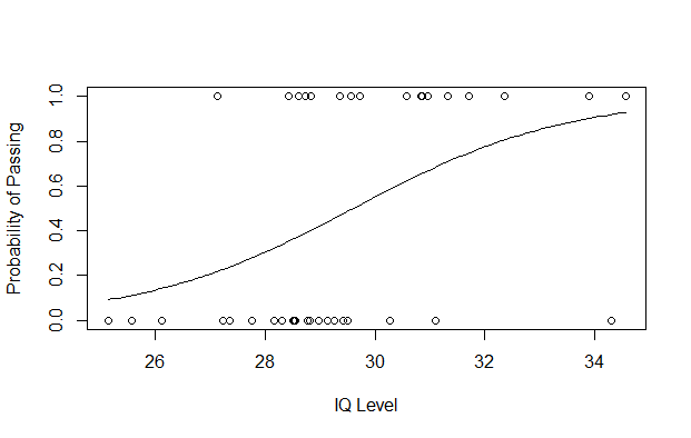
IQ Level Plot

R

# Based on fit to the regression model
points(IQ, fitted(g), pch=30)

# Summary of the regression model
summary(g)

Output:

Call:
glm(formula = result ~ IQ, family = binomial, data = df)

Deviance Residuals: 
    Min       1Q   Median       3Q      Max  
-2.2378  -0.9655  -0.4604   0.9368   1.7445  

Coefficients:
            Estimate Std. Error z value Pr(>|z|)  
(Intercept) -15.2593     6.3915  -2.387   0.0170 *
IQ            0.5153     0.2174   2.370   0.0178 *
---
Signif. codes:  0 ‘***’ 0.001 ‘**’ 0.01 ‘*’ 0.05 ‘.’ 0.1 ‘ ’ 1

(Dispersion parameter for binomial family taken to be 1)

    Null deviance: 55.352  on 39  degrees of freedom
Residual deviance: 47.411  on 38  degrees of freedom
AIC: 51.411

Number of Fisher Scoring iterations: 4