Register Allocations in Code Generation

Registers are the fastest locations in the memory hierarchy. But unfortunately, this resource is limited. It comes under the most constrained resources of the target processor. Register allocation is an NP-complete problem. However, this problem can be reduced to graph coloring to achieve allocation and assignment. Therefore a good register allocator computes an effective approximate solution to a hard problem. 

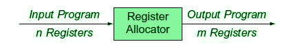
Figure – Input-Output 

The register allocator determines which values will reside in the register and which register will hold each of those values. It takes as its input a program with an arbitrary number of registers and produces a program with a finite register set that can fit into the target machine. (See image) 

Allocation vs Assignment:

Allocation –
Maps an unlimited namespace onto that register set of the target machine. 

• Reg. to Reg. Model: Maps virtual registers to physical registers but spills excess amount to memory.
• Mem. to Mem. Model: Maps some subset of the memory location to a set of names that models the physical register set.

Allocation ensures that code will fit the target machine’s reg. set at each instruction. 

Assignment –
Maps an allocated name set to the physical register set of the target machine.  

• Assumes allocation has been done so that code will fit into the set of physical registers.
• No more than ‘k’ values are designated into the registers, where ‘k’ is the no. of physical registers.

General register allocation is an NP-complete problem:

• Solved in polynomial time, when (no. of required registers) <= (no. of available physical registers).
• An assignment can be produced in linear time using Interval-Graph Coloring.

Local Register Allocation And Assignment:
Allocation just inside a basic block is called Local Reg. Allocation. Two approaches for local reg. allocation: Top-down approach and bottom-up approach. 

Top-Down Approach is a simple approach based on ‘Frequency Count’. Identify the values which should be kept in registers and which should be kept in memory. 

Algorithm:

1. Compute a priority for each virtual register.
2. Sort the registers into priority order.
3. Assign registers in priority order.
4. Rewrite the code.

Moving beyond single Blocks:

• More complicated because the control flow enters the picture.
• Liveness and Live Ranges: Live ranges consist of a set of definitions and uses that are related to each other as they i.e. no single register can be common in a such couple of instruction/data.

Following is a way to find out Live ranges in a block. A live range is represented as an interval [i,j], where i is the definition and j is the last use. 

Global Register Allocation and Assignment:
1. The main issue of a register allocator is minimizing the impact of spill code; 

• Execution time for spill code.
• Code space for spill operation.
• Data space for spilled values.

2. Global allocation can’t guarantee an optimal solution for the execution time of spill code. 
3. Prime differences between Local and Global Allocation: 

• The structure of a global live range is naturally more complex than the local one.
• Within a global live range, distinct references may execute a different number of times. (When basic blocks form a loop)

4. To make the decision about allocation and assignments, the global allocator mostly uses graph coloring by building an interference graph. 
5. Register allocator then attempts to construct a k-coloring for that graph where ‘k’ is the no. of physical registers. 

• In case, the compiler can’t directly construct a k-coloring for that graph, it modifies the underlying code by spilling some values to memory and tries again.
• Spilling actually simplifies that graph which ensures that the algorithm will halt.

6. Global Allocator uses several approaches, however, we’ll see top-down and bottom-up allocations strategies. Subproblems associated with the above approaches.  

• Discovering Global live ranges.
• Estimating Spilling Costs.
• Building an Interference graph.

Discovering Global Live Ranges:
How to discover Live range for a variable? 

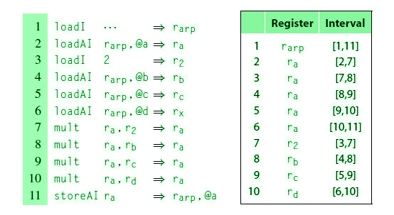
Figure – Discovering live ranges in a single block 

The above diagram explains everything properly. Let’s take the example of Rarp, it’s been initialized at program point 1 and its last usage is at program point 11. Therefore, the Live Range of Rarp i.e. Larp is [1,11]. Similarly, others follow up.  

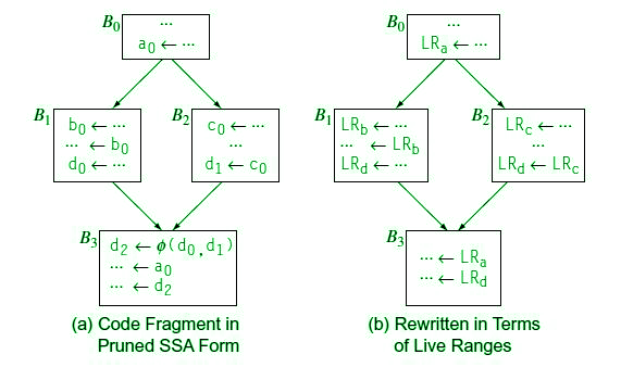
Figure – Discovering Live Ranges 

Estimating Global Spill Cost:

• Essential for taking a spill decision which includes – address computation, memory operation cost, and estimated execution frequency.
• For performance benefits, these spilled values are kept typically for the Activation records.
• Some embedded processors offer ScratchPad Memory to hold such spilled values.
• Negative Spill Cost: Consecutive load-store for a single address needs to be removed as it increases the burden, hence incurs negative spill cost.
• Infinite Spill Cost: A live range should have infinite spill cost if no other live range ends between its definition and its use.

Interference and Interference Graph:

Figure – Building Interference Graph from Live Ranges 

From the above diagram, it can be observed that the live range LRA starts in the first basic block and ends in the last basic block. Therefore it will share an edge with every other live Range i.e. Lrb, Lrc,Lrd. However, Lrb, Lrc, Lrd doesn’t overlap with any other live range except Lra so they are only sharing an edge with Lra. 

Building an Allocator:

• Note that a k-colorable graph finding is an NP-complete problem, so we need an approximation for this.
• Try with live range splitting into some non-trivial chunks (most used ones).

Top-Down Colouring: 

1. Tries to color live range in an order determined by some ranking functions i.e. priority based.
2. If no color is available for a live range, the allocator invokes either spilling or splitting to handle uncolored ones.
3. Live ranges having k or more neighbors are called constrained nodes and are difficult to handle.
4. The unconstrained nodes are comparatively easy to handle.
5. Handling Spills: When no color is found for some live ranges, spilling is needed to be done, but this may not be a final/ultimate solution of course.
6. Live Range Splitting: For uncolored ones, split the live range into sub-ranges, those may have fewer interferences than the original one so that some of them can be colored at least.

Chaitin’s Idea:

• Choose an arbitrary node of ( degree < k ) and put it in the stack.
• Remove that node and all its edges from the graph. (This may decrease the degree of some other nodes and cause some more nodes to have degree = k, some node has to be spilled.
• If no vertex needs to be spilled, successively pop vertices off the stack and color them in a color not used by neighbors. (reuse colors as far as possible).

Coalescing copies to reduce degree:
The compiler can use the interference graph to coalesce two live ranges. So by coalescing, what type of benefits can you get? 

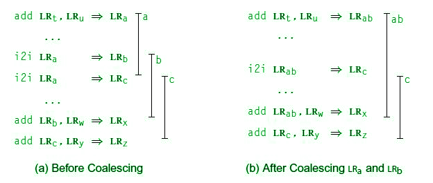
Figure – Coalescing Live Ranges 

Comparing Top-Down and Bottom-Up allocator:

• Top-down allocator could adopt the ‘spill and iterate’ philosophy used in bottom-up ones.
• ‘Spill and iterate’ trades additional compile time for an allocation that potentially, uses less spill code.
• Top-Down uses priority ranking to order all the constrained nodes. (However, it colors the unconstrained nodes in arbitrary order)
• Bottom-up constructs an order in which most nodes are colored in a graph where they are unconstrained.

Figure – Coalescing Live Ranges