Random Forest with Parallel Computing in R Programming
Last Updated :
02 Jul, 2020
Random Forest in R Programming is basically a bagging technique. From the name we can clearly interpret that this algorithm basically creates the forest with a lot of trees. It is a supervised classification algorithm.
In a general scenario, if we have a greater number of trees in a forest it gives the best aesthetic appeal to all and is counted as the best forest. The same is the scenario in random forest classifier, the higher the number of trees the better the accuracy and hence it turns out to be a better model. In a random forest, the same approach which you use in decision tree i.e. entropy and information gain is not going to be used. Here in the random forest, we draw random bootstrap samples from the training set.
Advantages of Random Forest:
- Good for Large Datasets to handle.
- The learning is fast and provides a high accuracy.
- Can handle plenty number of variables at once.
- Over-fitting is not a problem in this algorithm.
Disadvantages of Random Forest:
- Complexity is a major issue. Since the algorithm creates a number of trees and combines its output to produce the best output takes more computational time and resources.
- The time period usually for training a random forest model is greater since it generates a large number of trees.
Parallel Computing
Parallel Computing basically refers to the usage of two or more cores (or processors) at the same instance to get the solution of one problem existing. The main target here is to break the task into smaller sub-tasks and get them done simultaneously.
A simple mathematical example will clear the basic idea behind parallel computing:
Suppose we have the below expression to evaluate:
Z= 7a + 8b + 2c + 3d
Where, a = 1, b = 2, c = 9, d = 5.
Normal Process without parallel computing would be:
Step 1: Putting in the values of the variables.
Z = (7*1) + (8*2) + (2*9) + (3*5)
Step 2: Evaluating the expression:
Z = 7 + (8*2) + (2*9) + (3*5)
Step 3:
Z = 7 + 16 + (2*9) + (3*5)
Step 4:
Z = 7 + 16 + 18 + (3*5)
Step 5:
Z = 7 + 16 + 18 + 15
Step 6:
Z = 56
The same expression evaluation in the scenario of parallel computing would be as follows:
Step 1: Putting in the values of the variables.
Z = (7*1) + (8*2) + (2*9) + (3*5)
Step 2: Evaluating the expression:
Z = 7 + 16 + 18 + 15
Step 3:
Z = 56
So we can see the difference above that the evaluation of the expression is much faster in the second case.
So, I have taken a dataset of radar data. It consists of a total of 35 attributes. The 35th attribute is the target variable which is “g” or “b”. This target variable mainly represents the free electrons in the ionosphere. “g” is for Good” radar returns are those showing evidence of some type of structure in the ionosphere and “b” is for Bad” returns are those that do not; their signals pass through the ionosphere. So basically, it is a binary classification task. Let’s start with the coding part.
Loading the required libraries:
library(caret)
library(randomForest)
library(doParallel)
|
Reading the dataset:
datafile<-read.csv("C:/Users/prana/Downloads/ionosphere.data.csv")
datafile
|
Converting the target variable into factor variable with labels 0 and 1. Also check for missing values if any.
datafile$target0]
set.seed(100)
|
As there are no missing values, we have a clean dataset. Therefore, moving on to the model building part. Splitting the dataset into an 80:20 ratio i.e. training set and testing set respectively.
Trainingindex<-createDataPartition(datafile$target, p=0.8, list=FALSE)
trainingset<-datafile[Trainingindex, ]
testingset<-datafile[-Trainingindex, ]
|
Implementation of Random Forest without Parallel Computing
Now we will build a model normally and record the time taken for the same:
start.time<-proc.time()
model<-train(target~., data=trainingset, method='rf')
stop.time<-proc.time()
run.time<-stop.time -start.time
print(run.time)
|
Output:
user  system   elapsed
13.05   0.20     13.62
Implementation of Random Forest with Parallel Computing
Now building the model with parallel computing concept, loading the do Parallel library in R(here we have already loaded it in the beginning so no need to load it again). We can see the function makePSOCKcluster() which creates a set of copies of R running in parallel and communicating over sockets. The stopCluster() stops the engine node in the cluster in cl. We will also record the time taken to build the model by this approach.
cl<-makePSOCKcluster(5)
registerDoParallel(cl)
start.time<-proc.time()
model<-train(target~., data=trainingset, method='rf')
stop.time<-proc.time()
run.time<-stop.time -start.time
print(run.time)
stopCluster(cl)
|
Output:
user  system   elapsed
0.56    0.02      6.19
Comparison Table for Time Differences
So now formulating a table which will show us both the timings of the 2 approaches.
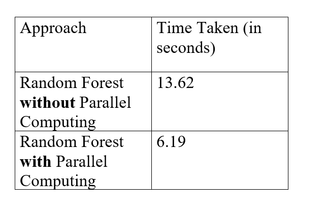
So, from the above table, we can conclude that with parallel computing the modeling process is 2.200323 (=13.62/6.19) times faster than the normal approach.
Like Article
Suggest improvement
Share your thoughts in the comments
Please Login to comment...