R-squared Regression Analysis in R Programming

For the prediction of one variable’s value(dependent variable) through other variables (independent variables) some models are used that are called regression models. For further calculating the accuracy of this prediction another mathematical tool is used, which is R-squared Regression Analysis or the coefficient of determination. The value of R-squared is between 0 and 1. If the coefficient of determination is 1 (or 100%) means that the prediction of the dependent variable has been perfect and accurate.

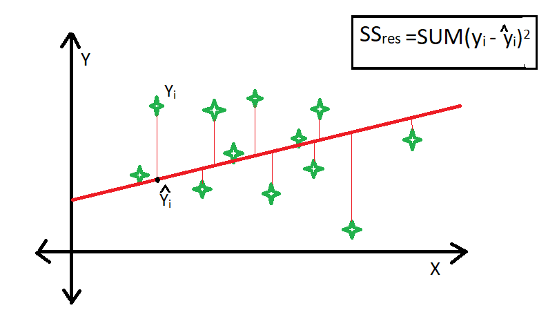
R-square is a comparison of the residual sum of squares (SS_res) with the total sum of squares(SS_tot). The residual sum of squares is calculated by the summation of squares of perpendicular distance between data points and the best-fitted line.

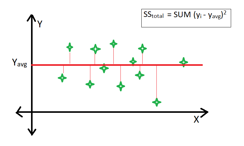
The total sum of squares is calculated by the summation of squares of perpendicular distance between data points and the average line.

Formula for R-squared Regression Analysis

The formula for R-squared Regression Analysis is given as follows,

where, : experimental values of the dependent variable : the average/mean : the fitted value

Find the Coefficient of Determination(R) in R

It is very easy to find out the Coefficient of Determination(R) in the R Programming Language.

The steps to follow are:

• Make a data frame in R.
• Calculate the linear regression model and save it in a new variable.
• The so calculated new variable’s summary has a coefficient of determination or R-squared parameter that needs to be extracted.

R

# Creating a data frame of exam marks
exam <- data.frame(name = c("ravi", "shaily",
                            "arsh", "monu"),
                math = c(87, 98, 67, 90),
                estimated = c(65, 87, 56, 100))

# Printing data frame
exam

Output:

    name math estimated
1   ravi   87        65
2 shaily   98        87
3   arsh   67        56
4   monu   90       100

Make model and calculate the summary of the model

R

# Calculating the linear regression model
model = lm(math~estimated, data = exam)

# Extracting R-squared parameter from summary
summary(model)

Output:

Call:
lm(formula = math ~ estimated, data = exam)
Residuals:
     1      2      3      4 
 7.421  7.566 -8.138 -6.848 
Coefficients:
            Estimate Std. Error t value Pr(>|t|)
(Intercept)  47.5074    24.0563   1.975    0.187
estimated     0.4934     0.3047   1.619    0.247
Residual standard error: 10.62 on 2 degrees of freedom
Multiple R-squared:  0.5673,    Adjusted R-squared:  0.3509 
F-statistic: 2.622 on 1 and 2 DF,  p-value: 0.2468

R

# Extracting R-squared parameter from summary
summary(model)$r.squared

Output:

[1] 0.5672797

Note: If the prediction is accurate the R-squared Regression value generated is 1.

• We’re using a linear regression model to understand the relationship between “math” scores and the variable “estimated.
• We’re using a linear regression model to understand the relationship between “math” scores and the variable “estimated.
• Residuals are the differences between actual “math” scores and what our model predicts. We have these differences for four observations.
• The intercept (where the line crosses the y-axis) is estimated to be 47.51. The coefficient for “estimated” is 0.49, suggesting that for each unit increase in “estimated,” the predicted “math” score increases by about 0.49 units.
• The p-values for both the intercept and “estimated” aren’t very low (0.187 and 0.247, respectively). This means that these coefficients may not be significantly different from zero at a standard significance level.
• This is an estimate of how spread out the residuals are, and here it’s about 10.62.
• The R-squared value of 0.5673 suggests that our model explains around 56.73% of the variation in “math” scores.
• This is a version of R-squared that considers the number of predictors. Here, it’s 0.3509 after adjusting.
• The F-statistic tests if our model is generally significant. A p-value of 0.2468 suggests the overall model might not be statistically significant.

R

# Creating a data frame of exam marks
exam <- data.frame(name = c("ravi", "shaily",
                            "arsh", "monu"),
                math = c(87, 98, 67, 90),
                estimated = c(87, 98, 67, 90))

# Printing data frame
exam

# Calculating the linear regression model
model = lm(math~estimated, data = exam)

# Extracting R-squared parameter from summary
summary(model)

Output:

    name math estimated
1   ravi   87        87
2 shaily   98        98
3   arsh   67        67
4   monu   90        90
Call:
lm(formula = math ~ estimated, data = exam)
Residuals:
         1          2          3          4 
 2.618e-15 -2.085e-15 -1.067e-15  5.330e-16 
Coefficients:
             Estimate Std. Error   t value Pr(>|t|)    
(Intercept) 0.000e+00  9.494e-15 0.000e+00        1    
estimated   1.000e+00  1.101e-16 9.086e+15   <2e-16 ***
---
Signif. codes:  0 ‘***’ 0.001 ‘**’ 0.01 ‘*’ 0.05 ‘.’ 0.1 ‘ ’ 1
Residual standard error: 2.512e-15 on 2 degrees of freedom
Multiple R-squared:      1,    Adjusted R-squared:      1 
F-statistic: 8.256e+31 on 1 and 2 DF,  p-value: < 2.2e-16

The summary function give all the information of the model.

Residual standard error: 2.512e-15 on 2 degrees of freedom
Multiple R-squared:      1,      Adjusted R-squared:      1 
F-statistic: 8.256e+31 on 1 and 2 DF,  p-value: < 2.2e-16

This model appears to be an impeccable fit for the data. The extremely tiny residual standard error indicates almost perfect prediction accuracy.

• The R-squared and adjusted R-squared values of 1 signify that the model explains 100% of the variation in “math” scores.
• The colossal F-statistic with an extremely low p-value reinforces the idea that the model is highly significant.

Limitation of Using R-square Method

• The value of r-square always increases or remains the same as new variables are added to the model, without detecting the significance of this newly added variable (i.e value of r-square never decreases on the addition of new attributes to the model). As a result, non-significant attributes can also be added to the model with an increase in r-square value.
• This is because SS_tot is always constant and the regression model tries to decrease the value of SS_res by finding some correlation with this new attribute and hence the overall value of r-square increases, which can lead to a poor regression model.