Quiver Plot in Matplotlib
Last Updated :
23 Feb, 2022
Quiver plot is basically a type of 2D plot which shows vector lines as arrows. This type of plots are useful in Electrical engineers to visualize electrical potential and show stress gradients in Mechanical engineering.
Creating a Quiver Plot
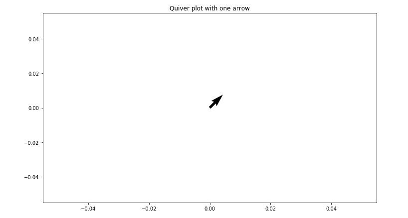
Let’s start creating a simple quiver plot containing one arrow which will explain how Matplotlib’s ax.quiver() function works. The ax.quiver() function takes four arguments:
Syntax:
ax.quiver(x_pos, y_pos, x_dir, y_dir, color)
Here x_pos and y_pos are the starting positions of the arrow while x_dir and y_dir are the directions of the arrow.
The below plot contains one quiver arrow starting at x_pos = 0 and y_pos = 0.The direction of the arrow is pointing towards up and the right at x_dir = 1 and y_dir = 1.
Example:
Python3
import numpy as np
import matplotlib.pyplot as plt
x_pos = 0
y_pos = 0
x_direct = 1
y_direct = 1
fig, ax = plt.subplots(figsize = (12, 7))
ax.quiver(x_pos, y_pos, x_direct, y_direct)
ax.set_title('Quiver plot with one arrow')
plt.show()
|
Output :
Quiver Plot with two arrows
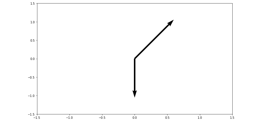
Let’s add another arrow to the plot passing through two starting points and two directions. By keeping the original arrow starting at origin(0, 0) and pointing towards up and to the right direction(1, 1), and create the second arrow starting at (0, 0) pointing down in direction(0, -1).To see the starting and ending point clearly, we will set axis limits to [-1.5, 1.5] using the method ax.axis() and passing the arguments in the form of [x_min, x_max, y_max, y_min] . By adding an additional argument scale=value to the ax.quiver() method we can manage the lengths of the arrows to look longer and show up better on the plot.
Example:
Python3
import numpy as np
import matplotlib.pyplot as plt
x_pos = [0, 0]
y_pos = [0, 0]
x_direct = [1, 0]
y_direct = [1, -1]
fig, ax = plt.subplots(figsize = (12, 7))
ax.quiver(x_pos, y_pos, x_direct, y_direct,
scale = 5)
ax.axis([-1.5, 1.5, -1.5, 1.5])
plt.show()
|
Output :
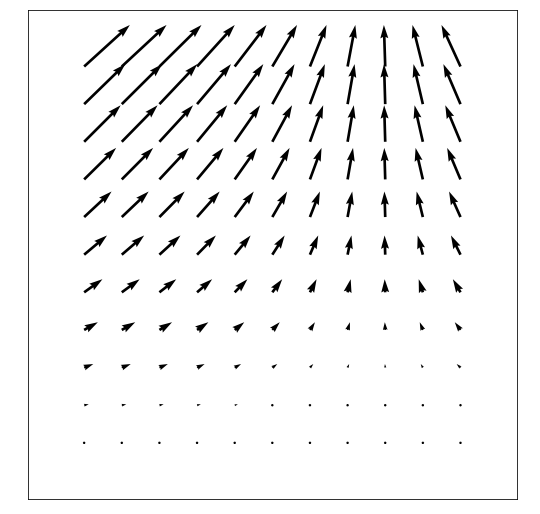
Quiver Plot using meshgrid
A quiver plot containing two arrows is a good start, but it is too slow and too long to add arrows to the quiver plot one by one.So to create a fully 2D surface of arrows we will use meshgrid() method of Numpy. First, create a set of arrays named X and Y which represent the starting positions of x and y respectively of each arrow on the quiver plot. The starting positions of x, y arrows can also be used to define the x and y components of each arrow direction. In the following plot u and v denote the array of directions of the quiver arrows and we will define the arrow direction based on the arrow starting point by using the equations below:
x_{direction} = cos(x_{starting \ point})
y_{direction} = sin(y_{starting \ point})
Example:
Python3
import numpy as np
import matplotlib.pyplot as plt
x = np.arange(0, 2.2, 0.2)
y = np.arange(0, 2.2, 0.2)
X, Y = np.meshgrid(x, y)
u = np.cos(X)*Y
v = np.sin(Y)*Y
fig, ax = plt.subplots(figsize =(14, 8))
ax.quiver(X, Y, u, v)
ax.xaxis.set_ticks([])
ax.yaxis.set_ticks([])
ax.axis([-0.3, 2.3, -0.3, 2.3])
ax.set_aspect('equal')
plt.show()
|
Output :
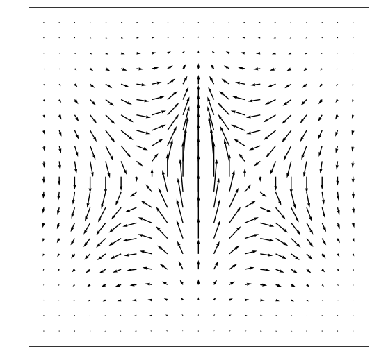
Quiver Plot using gradient
Let us create a quiver plot which shows the gradient function.The np, gradient() method of Numpy can be used to apply the gradient function to each arrow’s x, y starting position. The equation is used to create the following plot:
z = xe^{-x^2-y^2}
Example:
Python3
import numpy as np
import matplotlib.pyplot as plt
x = np.arange(-2, 2.2, 0.2)
y = np.arange(-2, 2.2, 0.2)
X, Y = np.meshgrid(x, y)
z = X * np.exp(-X**2-Y**2)
dx, dy = np.gradient(z)
fig, ax = plt.subplots(figsize =(9, 9))
ax.quiver(X, Y, dx, dy)
ax.xaxis.set_ticks([])
ax.yaxis.set_ticks([])
ax.set_aspect('equal')
plt.show()
|
Output :
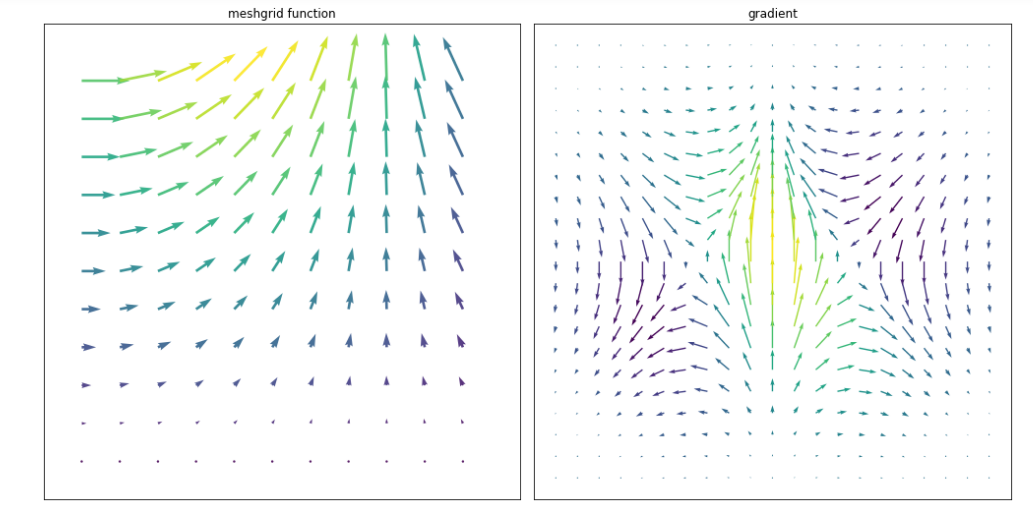
Coloring Quiver Plot
The ax.quiver() method of matplotlib library of python provides an optional attribute color that specifies the color of the arrow. The quiver color attribute requires the dimensions the same as the position and direction arrays.
Below is the code which modifies the quiver plots we made earlier:
Example 1:
Python3
import numpy as np
import matplotlib.pyplot as plt
fig, (ax1, ax2) = plt.subplots(1, 2, figsize =(14, 8))
x = np.arange(0, 2.2, 0.2)
y = np.arange(0, 2.2, 0.2)
X, Y = np.meshgrid(x, y)
u = np.cos(X)*Y
v = np.sin(y)*Y
n = -2
color = np.sqrt(((v-n)/2)*2 + ((u-n)/2)*2)
ax1.quiver(X, Y, u, v, color, alpha = 0.8)
ax1.xaxis.set_ticks([])
ax1.yaxis.set_ticks([])
ax1.axis([-0.2, 2.3, -0.2, 2.3])
ax1.set_aspect('equal')
ax1.set_title('meshgrid function')
x = np.arange(-2, 2.2, 0.2)
y = np.arange(-2, 2.2, 0.2)
X, Y = np.meshgrid(x, y)
z = X * np.exp(-X**2 -Y**2)
dx, dy = np.gradient(z)
n = -2
color = np.sqrt(((dx-n)/2)*2 + ((dy-n)/2)*2)
ax2.quiver(X, Y, dx, dy, color)
ax2.xaxis.set_ticks([])
ax2.yaxis.set_ticks([])
ax2.set_aspect('equal')
ax2.set_title('gradient')
plt.tight_layout()
plt.show()
|
Output :
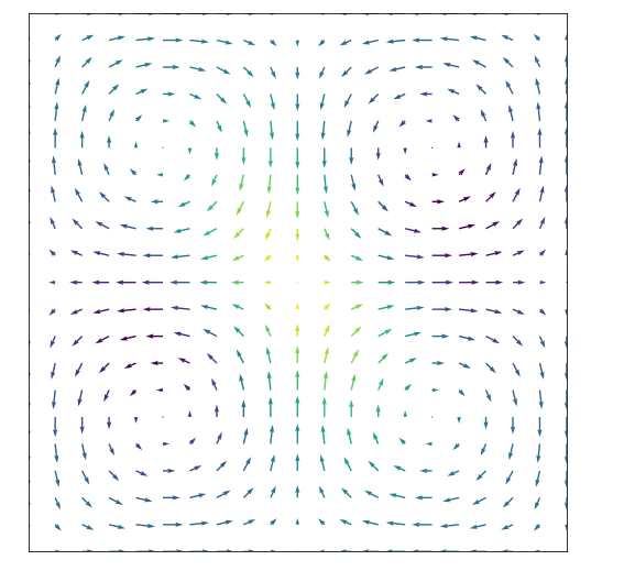
Example 2: Building a quiver plot of function  which defines the 2D field having four vertices as shown in the below plot:

Python3
import numpy as np
import matplotlib.pyplot as plt
x = np.arange(0, 2 * np.pi + 2 * np.pi / 20,
2 * np.pi / 20)
y = np.arange(0, 2 * np.pi + 2 * np.pi / 20,
2 * np.pi / 20)
X, Y = np.meshgrid(x, y)
u = np.sin(X)*np.cos(Y)
v = -np.cos(X)*np.sin(Y)
color = np.sqrt(((dx-n)/2)*2 + ((dy-n)/2)*2)
fig, ax = plt.subplots(figsize =(14, 9))
ax.quiver(X, Y, u, v, color, alpha = 1)
ax.xaxis.set_ticks([])
ax.yaxis.set_ticks([])
ax.axis([0, 2 * np.pi, 0, 2 * np.pi])
ax.set_aspect('equal')
plt.show()
|
Output :
Like Article
Suggest improvement
Share your thoughts in the comments
Please Login to comment...