Python – seaborn.lmplot() method

Seaborn is an amazing visualization library for statistical graphics plotting in Python. It provides beautiful default styles and color palettes to make statistical plots more attractive. It is built on the top of matplotlib library and also closely integrated to the data structures from pandas.

seaborn.Implot() method

seaborn.lmplot() method is used to draw a scatter plot onto a FacetGrid.

Syntax : seaborn.lmplot(x, y, data, hue=None, col=None, row=None, palette=None, col_wrap=None, height=5, aspect=1, markers=’o’, sharex=True, sharey=True, hue_order=None, col_order=None, row_order=None, legend=True, legend_out=True, x_estimator=None, x_bins=None, x_ci=’ci’, scatter=True, fit_reg=True, ci=95, n_boot=1000, units=None, seed=None, order=1, logistic=False, lowest=False, robust=False, logx=False, x_partial=None, y_partial=None, truncate=True, x_jitter=None, y_jitter=None, scatter_kws=None, line_kws=None, size=None)

Parameters : This method is accepting the following parameters that are described below: 

• x, y: ( optional) This parameters are column names in data.
• data : This parameter is DataFrame .
• hue, col, row : This parameters are define subsets of the data, which will be drawn on separate facets in the grid. See the *_order parameters to control the order of levels of this variable.
• palette: (optional) This parameter is palette name, list, or dict, Colors to use for the different levels of the hue variable. Should be something that can be interpreted by color_palette(), or a dictionary mapping hue levels to matplotlib colors.
• col_wrap : (optional) This parameter is of int type, “Wrap” the column variable at this width, so that the column facets span multiple rows. Incompatible with a row facet.
• height : (optional) This parameter is Height (in inches) of each facet.
• aspect : (optional) This parameter is Aspect ratio of each facet, so that aspect * height gives the width of each facet in inches.
• markers : (optional) This parameter is matplotlib marker code or list of marker codes, Markers for the scatterplot. If a list, each marker in the list will be used for each level of the hue variable.
• share{x, y} : (optional) This parameter is of bool type, ‘col’, or ‘row’, If true, the facets will share y axes across columns and/or x axes across rows.
• {hue, col, row}_order : (optional) This parameter is lists, Order for the levels of the faceting variables. By default, this will be the order that the levels appear in data or, if the variables are pandas categoricals, the category order.
• legend : (optional) This parameter accepting bool value, If True and there is a hue variable, add a legend.
• legend_out : (optional) This parameter accepting bool value, If True, the figure size will be extended, and the legend will be drawn outside the plot on the center right.
• x_estimator : (optional)This parameter is callable that maps vector -> scalar, Apply this function to each unique value of x and plot the resulting estimate. This is useful when x is a discrete variable. If x_ci is given, this estimate will be bootstrapped and a confidence interval will be drawn.
• x_bins : (optional) This parameter is int or vector, Bin the x variable into discrete bins and then estimate the central tendency and a confidence interval. This binning only influences how the scatter plot is drawn; the regression is still fit to the original data. This parameter is interpreted either as the number of evenly-sized (not necessary spaced) bins or the positions of the bin centers. When this parameter is used, it implies that the default of x_estimator is numpy.mean.
• x_ci : (optional) This parameter is “ci”, “sd”, int in [0, 100] or None, Size of the confidence interval used when plotting a central tendency for discrete values of x. If “ci”, defer to the value of the ci parameter. If “sd”, skip bootstrapping and show the standard deviation of the observations in each bin.
• scatter : (optional) This parameter accepting bool value . If True, draw a scatterplot with the underlying observations (or the x_estimator values).
• fit_reg : (optional) This parameter accepting bool value . If True, estimate and plot a regression model relating the x and y variables.
• ci : (optional) This parameter is int in [0, 100] or None, Size of the confidence interval for the regression estimate. This will be drawn using translucent bands around the regression line. The confidence interval is estimated using a bootstrap; for large datasets, it may be advisable to avoid that computation by setting this parameter to None.
• n_boot : (optional) This parameter is Number of bootstrap resamples used to estimate the ci. The default value attempts to balance time and stability; you may want to increase this value for “final” versions of plots.
• units : (optional) This parameter is variable name in data, If the x and y observations are nested within sampling units, those can be specified here. This will be taken into account when computing the confidence intervals by performing a multilevel bootstrap that resamples both units and observations (within unit). This does not otherwise influence how the regression is estimated or drawn.
• seed : (optional) This parameter is int, numpy.random.Generator, or numpy.random.RandomState, Seed or random number generator for reproducible bootstrapping.
• order : (optional) This parameter, order is greater than 1, use numpy.polyfit to estimate a polynomial regression.
• logistic : (optional) This parameter accepting bool value, If True, assume that y is a binary variable and use statsmodels to estimate a logistic regression model. Note that this is substantially more computationally intensive than linear regression, so you may wish to decrease the number of bootstrap resamples (n_boot) or set ci to None.
• lowest : (optional) This parameter accepting bool value, If True, use statsmodels to estimate a non-parametric lowest model (locally weighted linear regression). Note that confidence intervals cannot currently be drawn for this kind of model.
• robust : (optional) This parameter accepting bool value, If True, use statsmodels to estimate a robust regression. This will de-weight outliers. Note that this is substantially more computationally intensive than standard linear regression, so you may wish to decrease the number of bootstrap resamples (n_boot) or set ci to None.
• logx : (optional) This parameter accepting bool value. If True, estimate a linear regression of the form y ~ log(x), but plot the scatterplot and regression model in the input space. Note that x must be positive for this to work.
• {x, y}_partial : (optional) This parameter is strings in data or matrices, Confounding variables to regress out of the x or y variables before plotting.
• truncate : (optional) This parameter accepting bool value.If True, the regression line is bounded by the data limits. If False, it extends to the x axis limits.
• {x, y}_jitter : (optional) This parameter is Add uniform random noise of this size to either the x or y variables. The noise is added to a copy of the data after fitting the regression, and only influences the look of the scatterplot. This can be helpful when plotting variables that take discrete values.
• {scatter, line}_kws : (optional)dictionaries

Returns : This method returns the FacetGrid object with the plot on it for further tweaking. 

Note: For downloading the Tips dataset Click Here.

Below examples illustrate the lmplot() method of seaborn library.

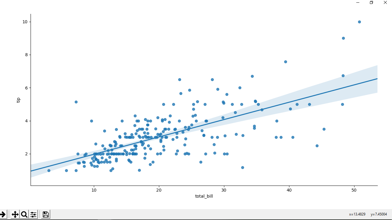
Example 1 : Scatter plot with regression line(by default).  

Python3

# importing the required library
import pandas as pd
import seaborn as sns
import matplotlib.pyplot as plt

# read a csv file
df = pd.read_csv('Tips.csv')

# scatter plot with regression
# line(by default)
sns.lmplot(x ='total_bill', y ='tip', data = df)

# Show the plot
plt.show()

Output :

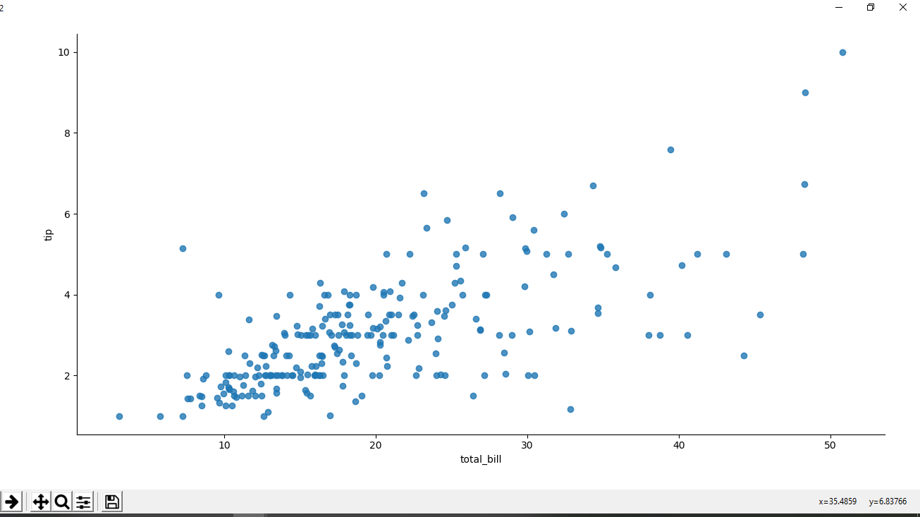
Example 2 : Scatter plot without regression line. 

Python3

# importing the required library
import pandas as pd
import seaborn as sns
import matplotlib.pyplot as plt

# read a csv file
df = pd.read_csv('Tips.csv')

# scatter plot without regression
# line.
sns.lmplot(x ='total_bill', y ='tip',
           fit_reg = False, data = df)

# Show the plot
plt.show()

Output :

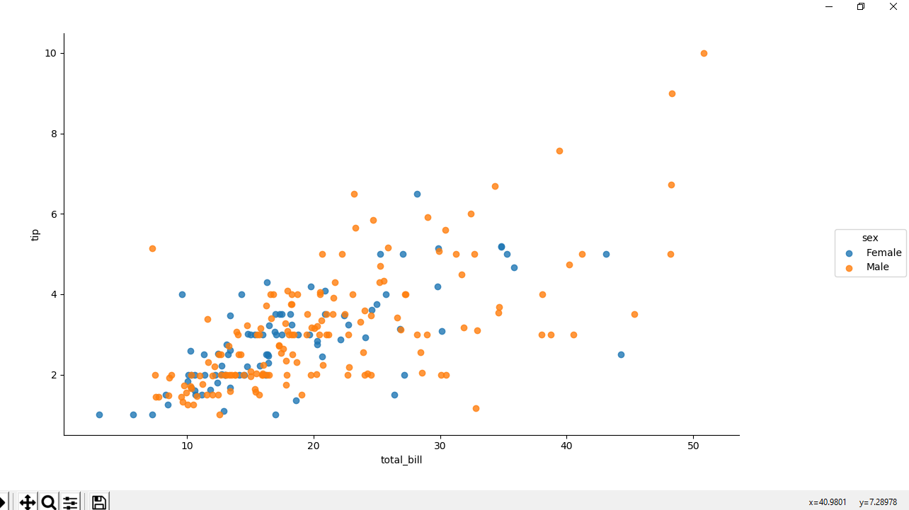
Example 3 : Scatter plot using hue attribute for coloring out points according to the sex. 

Python3

# importing the required library
import pandas as pd
import seaborn as sns
import matplotlib.pyplot as plt

# read a csv file
df = pd.read_csv('Tips.csv')

# scatter plot using hue attribute
# for colouring out points
# according to the sex
sns.lmplot(x ='total_bill', y ='tip',
          fit_reg = False, hue = 'sex',
          data = df)

# Show the plot
plt.show()

Output :