Python – Non-Central Chi-squared Distribution in Statistics

scipy.stats.ncx2() is a non-central chi-squared continuous random variable. It is inherited from the of generic methods as an instance of the rv_continuous class. It completes the methods with details specific for this particular distribution.

Parameters :

q : lower and upper tail probability
x : quantiles
loc : [optional]location parameter. Default = 0
scale : [optional]scale parameter. Default = 1
size : [tuple of ints, optional] shape or random variates.
moments : [optional] composed of letters [‘mvsk’]; ‘m’ = mean, ‘v’ = variance, ‘s’ = Fisher’s skew and ‘k’ = Fisher’s kurtosis. (default = ‘mv’).

Results : non-central chi-squared continuous random variable

Code #1 : Creating non-central chi-squared continuous random variable

# importing library

from scipy.stats import ncx2

numargs = ncx2.numargs
a, b = 4.32, 3.18
rv = ncx2(a, b)

print ("RV : \n", rv)

Output :

RV : 
 scipy.stats._distn_infrastructure.rv_frozen object at 0x000002A9D6E0FE08

Code #2 : non-central chi-squared continuous variates and probability distribution

import numpy as np
quantile = np.arange (0.01, 1, 0.1)

# Random Variates
R = ncx2.rvs(a, b)
print ("Random Variates : \n", R)

# PDF
R = ncx2.pdf(a, b, quantile)
print ("\nProbability Distribution : \n", R)

Output :

Random Variates : 
 1.452454339214702

Probability Distribution : 
 [0.10195838 0.10369453 0.10528707 0.1067405  0.10805931 0.1092479
 0.11031066 0.1112519  0.11207589 0.11278684]

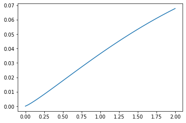
Code #3 : Graphical Representation.

import numpy as np
import matplotlib.pyplot as plt

distribution = np.linspace(0, np.minimum(rv.dist.b, 3))
print("Distribution : \n", distribution)

plot = plt.plot(distribution, rv.pdf(distribution))

Output :

Distribution : 
 [0.         0.04081633 0.08163265 0.12244898 0.16326531 0.20408163
 0.24489796 0.28571429 0.32653061 0.36734694 0.40816327 0.44897959
 0.48979592 0.53061224 0.57142857 0.6122449  0.65306122 0.69387755
 0.73469388 0.7755102  0.81632653 0.85714286 0.89795918 0.93877551
 0.97959184 1.02040816 1.06122449 1.10204082 1.14285714 1.18367347
 1.2244898  1.26530612 1.30612245 1.34693878 1.3877551  1.42857143
 1.46938776 1.51020408 1.55102041 1.59183673 1.63265306 1.67346939
 1.71428571 1.75510204 1.79591837 1.83673469 1.87755102 1.91836735
 1.95918367 2.        ]
 

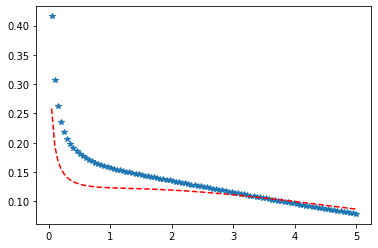
Code #4 : Varying Positional Arguments

import matplotlib.pyplot as plt
import numpy as np

x = np.linspace(0, 5, 100)

# Varying positional arguments
y1 = ncx2 .pdf(x, 1, 3)
y2 = ncx2 .pdf(x, 1, 4)
plt.plot(x, y1, "*", x, y2, "r--")

Output :