This tutorial is a beginner-friendly guide for learning data structures and algorithms using Python. In this article, we will discuss the in-built data structures such as lists, tuples, dictionaries, etc, and some user-defined data structures such as linked lists, trees, graphs, etc, and traversal as well as searching and sorting algorithms with the help of good and well-explained examples and practice questions.
Lists
Python Lists are ordered collections of data just like arrays in other programming languages. It allows different types of elements in the list. The implementation of Python List is similar to Vectors in C++ or ArrayList in JAVA. The costly operation is inserting or deleting the element from the beginning of the List as all the elements are needed to be shifted. Insertion and deletion at the end of the list can also become costly in the case where the preallocated memory becomes full.
Example: Creating Python List
Python3
List = [1, 2, 3, "GFG", 2.3]
print(List)
|
Output
[1, 2, 3, 'GFG', 2.3]
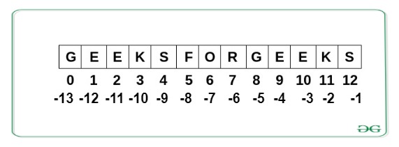
List elements can be accessed by the assigned index. In python starting index of the list, a sequence is 0 and the ending index is (if N elements are there) N-1.
Example: Python List Operations
Python3
List = ["Geeks", "For", "Geeks"]
print("\nList containing multiple values: ")
print(List)
List2 = [['Geeks', 'For'], ['Geeks']]
print("\nMulti-Dimensional List: ")
print(List2)
print("Accessing element from the list")
print(List[0])
print(List[2])
print("Accessing element using negative indexing")
print(List[-1])
print(List[-3])
|
Output
List containing multiple values:
['Geeks', 'For', 'Geeks']

Multi-Dimensional List:
[['Geeks', 'For'], ['Geeks']]
Accessing element from the list
Geeks
Geeks
Accessing element using negative indexing
Geeks
Geeks
Tuple
Python tuples are similar to lists but Tuples are immutable in nature i.e. once created it cannot be modified. Just like a List, a Tuple can also contain elements of various types.
In Python, tuples are created by placing a sequence of values separated by ‘comma’ with or without the use of parentheses for grouping of the data sequence.
Note: To create a tuple of one element there must be a trailing comma. For example, (8,) will create a tuple containing 8 as the element.
Example: Python Tuple Operations
Python3
Tuple = ('Geeks', 'For')
print("\nTuple with the use of String: ")
print(Tuple)
list1 = [1, 2, 4, 5, 6]
print("\nTuple using List: ")
Tuple = tuple(list1)
print("First element of tuple")
print(Tuple[0])
print("\nLast element of tuple")
print(Tuple[-1])
print("\nThird last element of tuple")
print(Tuple[-3])
|
Output
Tuple with the use of String:
('Geeks', 'For')

Tuple using List:
First element of tuple
1

Last element of tuple
6

Third last element of tuple
4
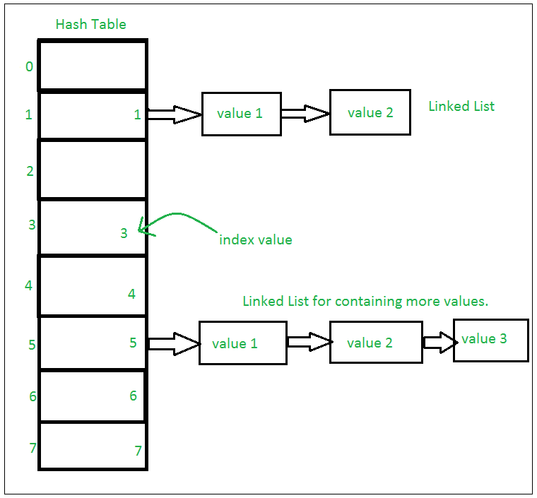
Set
Python set is a mutable collection of data that does not allow any duplication. Sets are basically used to include membership testing and eliminating duplicate entries. The data structure used in this is Hashing, a popular technique to perform insertion, deletion, and traversal in O(1) on average.
If Multiple values are present at the same index position, then the value is appended to that index position, to form a Linked List. In, CPython Sets are implemented using a dictionary with dummy variables, where key beings the members set with greater optimizations to the time complexity.
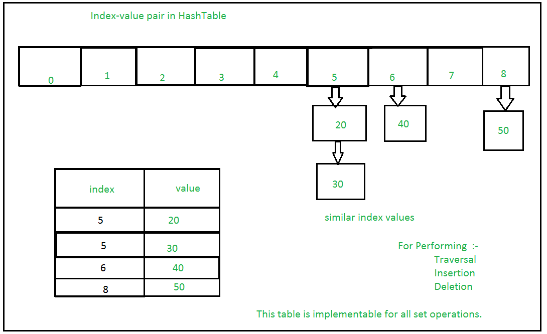
Set Implementation:
Sets with Numerous operations on a single HashTable:
Example: Python Set Operations
Python3
Set = set([1, 2, 'Geeks', 4, 'For', 6, 'Geeks'])
print("\nSet with the use of Mixed Values")
print(Set)
print("\nElements of set: ")
for i in Set:
print(i, end =" ")
print()
print("Geeks" in Set)
|
Output
Set with the use of Mixed Values
{1, 2, 4, 6, 'For', 'Geeks'}

Elements of set:
1 2 4 6 For Geeks
True
Frozen Sets
Frozen sets in Python are immutable objects that only support methods and operators that produce a result without affecting the frozen set or sets to which they are applied. While elements of a set can be modified at any time, elements of the frozen set remain the same after creation.
Example: Python Frozen set
Python3
normal_set = set(["a", "b","c"])
print("Normal Set")
print(normal_set)
frozen_set = frozenset(["e", "f", "g"])
print("\nFrozen Set")
print(frozen_set)
|
Output
Normal Set
{'a', 'b', 'c'}

Frozen Set
frozenset({'f', 'g', 'e'})
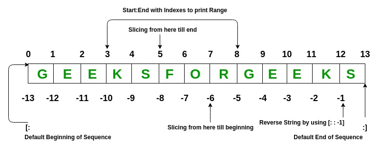
String
Python Strings is the immutable array of bytes representing Unicode characters. Python does not have a character data type, a single character is simply a string with a length of 1.
Note: As strings are immutable, modifying a string will result in creating a new copy.
Example: Python Strings Operations
Python3
String = "Welcome to GeeksForGeeks"
print("Creating String: ")
print(String)
print("\nFirst character of String is: ")
print(String[0])
print("\nLast character of String is: ")
print(String[-1])
|
Output
Creating String:
Welcome to GeeksForGeeks

First character of String is:
W

Last character of String is:
s
Dictionary
Python dictionary is an unordered collection of data that stores data in the format of key:value pair. It is like hash tables in any other language with the time complexity of O(1). Indexing of Python Dictionary is done with the help of keys. These are of any hashable type i.e. an object whose can never change like strings, numbers, tuples, etc. We can create a dictionary by using curly braces ({}) or dictionary comprehension.
Example: Python Dictionary Operations
Python3
Dict = {'Name': 'Geeks', 1: [1, 2, 3, 4]}
print("Creating Dictionary: ")
print(Dict)
print("Accessing a element using key:")
print(Dict['Name'])
print("Accessing a element using get:")
print(Dict.get(1))
myDict = {x: x**2 for x in [1,2,3,4,5]}
print(myDict)
|
Output
Creating Dictionary:
{'Name': 'Geeks', 1: [1, 2, 3, 4]}
Accessing a element using key:
Geeks
Accessing a element using get:
[1, 2, 3, 4]
{1: 1, 2: 4, 3: 9, 4: 16, 5: 25}
Matrix
A matrix is a 2D array where each element is of strictly the same size. To create a matrix we will be using the NumPy package.
Example: Python NumPy Matrix Operations
Python3
import numpy as np
a = np.array([[1,2,3,4],[4,55,1,2],
[8,3,20,19],[11,2,22,21]])
m = np.reshape(a,(4, 4))
print(m)
print("\nAccessing Elements")
print(a[1])
print(a[2][0])
m = np.append(m,[[1, 15,13,11]],0)
print("\nAdding Element")
print(m)
m = np.delete(m,[1],0)
print("\nDeleting Element")
print(m)
|
Output
[[ 1  2  3  4]
 [ 4 55  1  2]
 [ 8  3 20 19]
 [11  2 22 21]]

Accessing Elements
[ 4 55  1  2]
8

Adding Element
[[ 1  2  3  4]
 [ 4 55  1  2]
 [ 8  3 20 19]
 [11  2 22 21]
 [ 1 15 13 11]]

Deleting Element
[[ 1  2  3  4]
 [ 8  3 20 19]
 [11  2 22 21]
 [ 1 15 13 11]]
Bytearray
Python Bytearray gives a mutable sequence of integers in the range 0 <= x < 256.
Example: Python Bytearray Operations
Python3
a = bytearray((12, 8, 25, 2))
print("Creating Bytearray:")
print(a)
print("\nAccessing Elements:", a[1])
a[1] = 3
print("\nAfter Modifying:")
print(a)
a.append(30)
print("\nAfter Adding Elements:")
print(a)
|
Output
Creating Bytearray:
bytearray(b'\x0c\x08\x19\x02')

Accessing Elements: 8

After Modifying:
bytearray(b'\x0c\x03\x19\x02')

After Adding Elements:
bytearray(b'\x0c\x03\x19\x02\x1e')
Linked List
A linked list is a linear data structure, in which the elements are not stored at contiguous memory locations. The elements in a linked list are linked using pointers as shown in the below image:
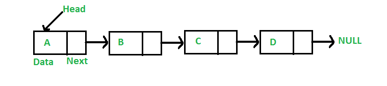
A linked list is represented by a pointer to the first node of the linked list. The first node is called the head. If the linked list is empty, then the value of the head is NULL. Each node in a list consists of at least two parts:
- Data
- Pointer (Or Reference) to the next node
Example: Defining Linked List in Python
Python3
class Node:
def __init__(self, data):
self.data = data
self.next = None
class LinkedList:
def __init__(self):
self.head = None
|
Let us create a simple linked list with 3 nodes.
Python3
class Node:
def __init__(self, data):
self.data = data
self.next = None
class LinkedList:
def __init__(self):
self.head = None
if __name__=='__main__':
llist = LinkedList()
llist.head = Node(1)
second = Node(2)
third = Node(3)
llist.head.next = second;
second.next = third;
|
Linked List Traversal
In the previous program, we have created a simple linked list with three nodes. Let us traverse the created list and print the data of each node. For traversal, let us write a general-purpose function printList() that prints any given list.
Python3
class Node:
def __init__(self, data):
self.data = data
self.next = None
class LinkedList:
def __init__(self):
self.head = None
def printList(self):
temp = self.head
while (temp):
print (temp.data)
temp = temp.next
if __name__=='__main__':
llist = LinkedList()
llist.head = Node(1)
second = Node(2)
third = Node(3)
llist.head.next = second;
second.next = third;
llist.printList()
|
More articles on Linked List
>>> More
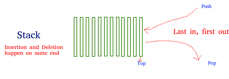
Stack
A stack is a linear data structure that stores items in a Last-In/First-Out (LIFO) or First-In/Last-Out (FILO) manner. In stack, a new element is added at one end and an element is removed from that end only. The insert and delete operations are often called push and pop.
The functions associated with stack are:
- empty() – Returns whether the stack is empty – Time Complexity: O(1)
- size() – Returns the size of the stack – Time Complexity: O(1)
- top() – Returns a reference to the topmost element of the stack – Time Complexity: O(1)
- push(a) – Inserts the element ‘a’ at the top of the stack – Time Complexity: O(1)
- pop() – Deletes the topmost element of the stack – Time Complexity: O(1)
Python3
stack = []
stack.append('g')
stack.append('f')
stack.append('g')
print('Initial stack')
print(stack)
print('\nElements popped from stack:')
print(stack.pop())
print(stack.pop())
print(stack.pop())
print('\nStack after elements are popped:')
print(stack)
|
Output
Initial stack
['g', 'f', 'g']
Elements popped from stack:
g
f
g
Stack after elements are popped:
[]
More articles on Stack
>>> More
Queue
As a stack, the queue is a linear data structure that stores items in a First In First Out (FIFO) manner. With a queue, the least recently added item is removed first. A good example of the queue is any queue of consumers for a resource where the consumer that came first is served first.
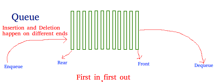
Operations associated with queue are:
- Enqueue: Adds an item to the queue. If the queue is full, then it is said to be an Overflow condition – Time Complexity: O(1)
- Dequeue: Removes an item from the queue. The items are popped in the same order in which they are pushed. If the queue is empty, then it is said to be an Underflow condition – Time Complexity: O(1)
- Front: Get the front item from queue – Time Complexity: O(1)
- Rear: Get the last item from queue – Time Complexity: O(1)
Python3
queue = []
queue.append('g')
queue.append('f')
queue.append('g')
print("Initial queue")
print(queue)
print("\nElements dequeued from queue")
print(queue.pop(0))
print(queue.pop(0))
print(queue.pop(0))
print("\nQueue after removing elements")
print(queue)
|
Output
Initial queue
['g', 'f', 'g']
Elements dequeued from queue
g
f
g
Queue after removing elements
[]
More articles on Queue
Priority Queue
Priority Queues are abstract data structures where each data/value in the queue has a certain priority. For example, In airlines, baggage with the title “Business” or “First-class” arrives earlier than the rest. Priority Queue is an extension of the queue with the following properties.
- An element with high priority is dequeued before an element with low priority.
- If two elements have the same priority, they are served according to their order in the queue.
Python3
class PriorityQueue(object):
def __init__(self):
self.queue = []
def __str__(self):
return ' '.join([str(i) for i in self.queue])
def isEmpty(self):
return len(self.queue) == 0
def insert(self, data):
self.queue.append(data)
def delete(self):
try:
max = 0
for i in range(len(self.queue)):
if self.queue[i] > self.queue[max]:
max = i
item = self.queue[max]
del self.queue[max]
return item
except IndexError:
print()
exit()
if __name__ == '__main__':
myQueue = PriorityQueue()
myQueue.insert(12)
myQueue.insert(1)
myQueue.insert(14)
myQueue.insert(7)
print(myQueue)
while not myQueue.isEmpty():
print(myQueue.delete())
|
Output
12 1 14 7
14
12
7
1
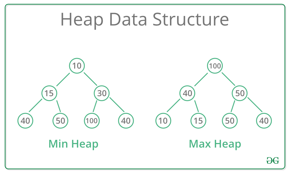
Heap
heapq module in Python provides the heap data structure that is mainly used to represent a priority queue. The property of this data structure is that it always gives the smallest element (min heap) whenever the element is popped. Whenever elements are pushed or popped, heap structure is maintained. The heap[0] element also returns the smallest element each time. It supports the extraction and insertion of the smallest element in the O(log n) times.
Generally, Heaps can be of two types:
- Max-Heap: In a Max-Heap the key present at the root node must be greatest among the keys present at all of it’s children. The same property must be recursively true for all sub-trees in that Binary Tree.
- Min-Heap: In a Min-Heap the key present at the root node must be minimum among the keys present at all of it’s children. The same property must be recursively true for all sub-trees in that Binary Tree.
Python3
import heapq
li = [5, 7, 9, 1, 3]
heapq.heapify(li)
print ("The created heap is : ",end="")
print (list(li))
heapq.heappush(li,4)
print ("The modified heap after push is : ",end="")
print (list(li))
print ("The popped and smallest element is : ",end="")
print (heapq.heappop(li))
|
Output
The created heap is : [1, 3, 9, 7, 5]
The modified heap after push is : [1, 3, 4, 7, 5, 9]
The popped and smallest element is : 1
More Articles on Heap
>>> More
Binary Tree
A tree is a hierarchical data structure that looks like the below figure –
tree
----
j <-- root
/ \
f k
/ \ \
a h z <-- leaves
The topmost node of the tree is called the root whereas the bottommost nodes or the nodes with no children are called the leaf nodes. The nodes that are directly under a node are called its children and the nodes that are directly above something are called its parent.
A binary tree is a tree whose elements can have almost two children. Since each element in a binary tree can have only 2 children, we typically name them the left and right children. A Binary Tree node contains the following parts.
- Data
- Pointer to left child
- Pointer to the right child
Example: Defining Node Class
Python3
class Node:
def __init__(self,key):
self.left = None
self.right = None
self.val = key
|
Now let’s create a tree with 4 nodes in Python. Let’s assume the tree structure looks like below –
tree
----
1 <-- root
/ \
2 3
/
4
Example: Adding data to the tree
Python3
class Node:
def __init__(self,key):
self.left = None
self.right = None
self.val = key
root = Node(1)
root.left = Node(2);
root.right = Node(3);
root.left.left = Node(4);
|
Tree Traversal
Trees can be traversed in different ways. Following are the generally used ways for traversing trees. Let us consider the below tree –
tree
----
1 <-- root
/ \
2 3
/ \
4 5
Depth First Traversals:
- Inorder (Left, Root, Right) : 4 2 5 1 3
- Preorder (Root, Left, Right) : 1 2 4 5 3
- Postorder (Left, Right, Root) : 4 5 2 3 1
Algorithm Inorder(tree)
- Traverse the left subtree, i.e., call Inorder(left-subtree)
- Visit the root.
- Traverse the right subtree, i.e., call Inorder(right-subtree)
Algorithm Preorder(tree)
- Visit the root.
- Traverse the left subtree, i.e., call Preorder(left-subtree)
- Traverse the right subtree, i.e., call Preorder(right-subtree)
Algorithm Postorder(tree)
- Traverse the left subtree, i.e., call Postorder(left-subtree)
- Traverse the right subtree, i.e., call Postorder(right-subtree)
- Visit the root.
Python3
class Node:
def __init__(self, key):
self.left = None
self.right = None
self.val = key
def printInorder(root):
if root:
printInorder(root.left)
print(root.val),
printInorder(root.right)
def printPostorder(root):
if root:
printPostorder(root.left)
printPostorder(root.right)
print(root.val),
def printPreorder(root):
if root:
print(root.val),
printPreorder(root.left)
printPreorder(root.right)
root = Node(1)
root.left = Node(2)
root.right = Node(3)
root.left.left = Node(4)
root.left.right = Node(5)
print("Preorder traversal of binary tree is")
printPreorder(root)
print("\nInorder traversal of binary tree is")
printInorder(root)
print("\nPostorder traversal of binary tree is")
printPostorder(root)
|
Output
Preorder traversal of binary tree is
1
2
4
5
3
Inorder traversal of binary tree is
4
2
5
1
3
Postorder traversal of binary tree is
4
5
2
3
1
Time Complexity – O(n)
Breadth-First or Level Order Traversal
Level order traversal of a tree is breadth-first traversal for the tree. The level order traversal of the above tree is 1 2 3 4 5.
For each node, first, the node is visited and then its child nodes are put in a FIFO queue. Below is the algorithm for the same –
- Create an empty queue q
- temp_node = root /*start from root*/
- Loop while temp_node is not NULL
- print temp_node->data.
- Enqueue temp_node’s children (first left then right children) to q
- Dequeue a node from q
Python3
class Node:
def __init__(self ,key):
self.data = key
self.left = None
self.right = None
def printLevelOrder(root):
if root is None:
return
queue = []
queue.append(root)
while(len(queue) > 0):
print (queue[0].data)
node = queue.pop(0)
if node.left is not None:
queue.append(node.left)
if node.right is not None:
queue.append(node.right)
root = Node(1)
root.left = Node(2)
root.right = Node(3)
root.left.left = Node(4)
root.left.right = Node(5)
print ("Level Order Traversal of binary tree is -")
printLevelOrder(root)
|
Output
Level Order Traversal of binary tree is -
1
2
3
4
5
Time Complexity: O(n)
More articles on Binary Tree
>>> More
Binary Search Tree
Binary Search Tree is a node-based binary tree data structure that has the following properties:
- The left subtree of a node contains only nodes with keys lesser than the node’s key.
- The right subtree of a node contains only nodes with keys greater than the node’s key.
- The left and right subtree each must also be a binary search tree.

The above properties of the Binary Search Tree provide an ordering among keys so that the operations like search, minimum and maximum can be done fast. If there is no order, then we may have to compare every key to search for a given key.
Searching Element
- Start from the root.
- Compare the searching element with root, if less than root, then recurse for left, else recurse for right.
- If the element to search is found anywhere, return true, else return false.
Python3
def search(root,key):
if root is None or root.val == key:
return root
if root.val < key:
return search(root.right,key)
return search(root.left,key)
|
Insertion of a key
- Start from the root.
- Compare the inserting element with root, if less than root, then recurse for left, else recurse for right.
- After reaching the end, just insert that node at left(if less than current) else right.
Python3
class Node:
def __init__(self, key):
self.left = None
self.right = None
self.val = key
def insert(root, key):
if root is None:
return Node(key)
else:
if root.val == key:
return root
elif root.val < key:
root.right = insert(root.right, key)
else:
root.left = insert(root.left, key)
return root
def inorder(root):
if root:
inorder(root.left)
print(root.val)
inorder(root.right)
r = Node(50)
r = insert(r, 30)
r = insert(r, 20)
r = insert(r, 40)
r = insert(r, 70)
r = insert(r, 60)
r = insert(r, 80)
inorder(r)
|
Output
20
30
40
50
60
70
80
More Articles on Binary Search Tree
>>> More
Graphs
A graph is a nonlinear data structure consisting of nodes and edges. The nodes are sometimes also referred to as vertices and the edges are lines or arcs that connect any two nodes in the graph. More formally a Graph can be defined as a Graph consisting of a finite set of vertices(or nodes) and a set of edges that connect a pair of nodes.
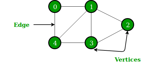
In the above Graph, the set of vertices V = {0,1,2,3,4} and the set of edges E = {01, 12, 23, 34, 04, 14, 13}. The following two are the most commonly used representations of a graph.
- Adjacency Matrix
- Adjacency List
Adjacency Matrix
Adjacency Matrix is a 2D array of size V x V where V is the number of vertices in a graph. Let the 2D array be adj[][], a slot adj[i][j] = 1 indicates that there is an edge from vertex i to vertex j. The adjacency matrix for an undirected graph is always symmetric. Adjacency Matrix is also used to represent weighted graphs. If adj[i][j] = w, then there is an edge from vertex i to vertex j with weight w.
Python3
class Graph:
def __init__(self,numvertex):
self.adjMatrix = [[-1]*numvertex for x in range(numvertex)]
self.numvertex = numvertex
self.vertices = {}
self.verticeslist =[0]*numvertex
def set_vertex(self,vtx,id):
if 0<=vtx<=self.numvertex:
self.vertices[id] = vtx
self.verticeslist[vtx] = id
def set_edge(self,frm,to,cost=0):
frm = self.vertices[frm]
to = self.vertices[to]
self.adjMatrix[frm][to] = cost
self.adjMatrix[to][frm] = cost
def get_vertex(self):
return self.verticeslist
def get_edges(self):
edges=[]
for i in range (self.numvertex):
for j in range (self.numvertex):
if (self.adjMatrix[i][j]!=-1):
edges.append((self.verticeslist[i],self.verticeslist[j],self.adjMatrix[i][j]))
return edges
def get_matrix(self):
return self.adjMatrix
G =Graph(6)
G.set_vertex(0,'a')
G.set_vertex(1,'b')
G.set_vertex(2,'c')
G.set_vertex(3,'d')
G.set_vertex(4,'e')
G.set_vertex(5,'f')
G.set_edge('a','e',10)
G.set_edge('a','c',20)
G.set_edge('c','b',30)
G.set_edge('b','e',40)
G.set_edge('e','d',50)
G.set_edge('f','e',60)
print("Vertices of Graph")
print(G.get_vertex())
print("Edges of Graph")
print(G.get_edges())
print("Adjacency Matrix of Graph")
print(G.get_matrix())
|
Output
Vertices of Graph
[‘a’, ‘b’, ‘c’, ‘d’, ‘e’, ‘f’]
Edges of Graph
[(‘a’, ‘c’, 20), (‘a’, ‘e’, 10), (‘b’, ‘c’, 30), (‘b’, ‘e’, 40), (‘c’, ‘a’, 20), (‘c’, ‘b’, 30), (‘d’, ‘e’, 50), (‘e’, ‘a’, 10), (‘e’, ‘b’, 40), (‘e’, ‘d’, 50), (‘e’, ‘f’, 60), (‘f’, ‘e’, 60)]
Adjacency Matrix of Graph
[[-1, -1, 20, -1, 10, -1], [-1, -1, 30, -1, 40, -1], [20, 30, -1, -1, -1, -1], [-1, -1, -1, -1, 50, -1], [10, 40, -1, 50, -1, 60], [-1, -1, -1, -1, 60, -1]]
Adjacency List
An array of lists is used. The size of the array is equal to the number of vertices. Let the array be an array[]. An entry array[i] represents the list of vertices adjacent to the ith vertex. This representation can also be used to represent a weighted graph. The weights of edges can be represented as lists of pairs. Following is the adjacency list representation of the above graph.

Python3
class AdjNode:
def __init__(self, data):
self.vertex = data
self.next = None
class Graph:
def __init__(self, vertices):
self.V = vertices
self.graph = [None] * self.V
def add_edge(self, src, dest):
node = AdjNode(dest)
node.next = self.graph[src]
self.graph[src] = node
node = AdjNode(src)
node.next = self.graph[dest]
self.graph[dest] = node
def print_graph(self):
for i in range(self.V):
print("Adjacency list of vertex {}\n head".format(i), end="")
temp = self.graph[i]
while temp:
print(" -> {}".format(temp.vertex), end="")
temp = temp.next
print(" \n")
if __name__ == "__main__":
V = 5
graph = Graph(V)
graph.add_edge(0, 1)
graph.add_edge(0, 4)
graph.add_edge(1, 2)
graph.add_edge(1, 3)
graph.add_edge(1, 4)
graph.add_edge(2, 3)
graph.add_edge(3, 4)
graph.print_graph()
|
Output
Adjacency list of vertex 0
 head -> 4 -> 1

Adjacency list of vertex 1
 head -> 4 -> 3 -> 2 -> 0

Adjacency list of vertex 2
 head -> 3 -> 1

Adjacency list of vertex 3
 head -> 4 -> 2 -> 1

Adjacency list of vertex 4
 head -> 3 -> 1 -> 0
Graph Traversal
Breadth-First Search or BFS
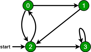
Breadth-First Traversal for a graph is similar to Breadth-First Traversal of a tree. The only catch here is, unlike trees, graphs may contain cycles, so we may come to the same node again. To avoid processing a node more than once, we use a boolean visited array. For simplicity, it is assumed that all vertices are reachable from the starting vertex.
For example, in the following graph, we start traversal from vertex 2. When we come to vertex 0, we look for all adjacent vertices of it. 2 is also an adjacent vertex of 0. If we don’t mark visited vertices, then 2 will be processed again and it will become a non-terminating process. A Breadth-First Traversal of the following graph is 2, 0, 3, 1.
Python3
from collections import defaultdict
class Graph:
def __init__(self):
self.graph = defaultdict(list)
def addEdge(self,u,v):
self.graph[u].append(v)
def BFS(self, s):
visited = [False] * (max(self.graph) + 1)
queue = []
queue.append(s)
visited[s] = True
while queue:
s = queue.pop(0)
print (s, end = " ")
for i in self.graph[s]:
if visited[i] == False:
queue.append(i)
visited[i] = True
g = Graph()
g.addEdge(0, 1)
g.addEdge(0, 2)
g.addEdge(1, 2)
g.addEdge(2, 0)
g.addEdge(2, 3)
g.addEdge(3, 3)
print ("Following is Breadth First Traversal"
" (starting from vertex 2)")
g.BFS(2)
|
Output
Following is Breadth First Traversal (starting from vertex 2)
2 0 3 1
Time Complexity: O(V+E) where V is the number of vertices in the graph and E is the number of edges in the graph.
Depth First Search or DFS
Depth First Traversal for a graph is similar to Depth First Traversal of a tree. The only catch here is, unlike trees, graphs may contain cycles, a node may be visited twice. To avoid processing a node more than once, use a boolean visited array.
Algorithm:
- Create a recursive function that takes the index of the node and a visited array.
- Mark the current node as visited and print the node.
- Traverse all the adjacent and unmarked nodes and call the recursive function with the index of the adjacent node.
Python3
from collections import defaultdict
class Graph:
def __init__(self):
self.graph = defaultdict(list)
def addEdge(self, u, v):
self.graph[u].append(v)
def DFSUtil(self, v, visited):
visited.add(v)
print(v, end=' ')
for neighbour in self.graph[v]:
if neighbour not in visited:
self.DFSUtil(neighbour, visited)
def DFS(self, v):
visited = set()
self.DFSUtil(v, visited)
g = Graph()
g.addEdge(0, 1)
g.addEdge(0, 2)
g.addEdge(1, 2)
g.addEdge(2, 0)
g.addEdge(2, 3)
g.addEdge(3, 3)
print("Following is DFS from (starting from vertex 2)")
g.DFS(2)
|
Output
Following is DFS from (starting from vertex 2)
2 0 1 3
More articles on graph
>>> More
Recursion
The process in which a function calls itself directly or indirectly is called recursion and the corresponding function is called a recursive function. Using the recursive algorithms, certain problems can be solved quite easily. Examples of such problems are Towers of Hanoi (TOH), Inorder/Preorder/Postorder Tree Traversals, DFS of Graph, etc.
What is the base condition in recursion?
In the recursive program, the solution to the base case is provided and the solution of the bigger problem is expressed in terms of smaller problems.
def fact(n):

    # base case
    if (n < = 1)
        return 1
    else
        return n*fact(n-1)
In the above example, base case for n < = 1 is defined and larger value of number can be solved by converting to smaller one till base case is reached.
How memory is allocated to different function calls in recursion?
When any function is called from main(), the memory is allocated to it on the stack. A recursive function calls itself, the memory for a called function is allocated on top of memory allocated to the calling function and a different copy of local variables is created for each function call. When the base case is reached, the function returns its value to the function by whom it is called and memory is de-allocated and the process continues.
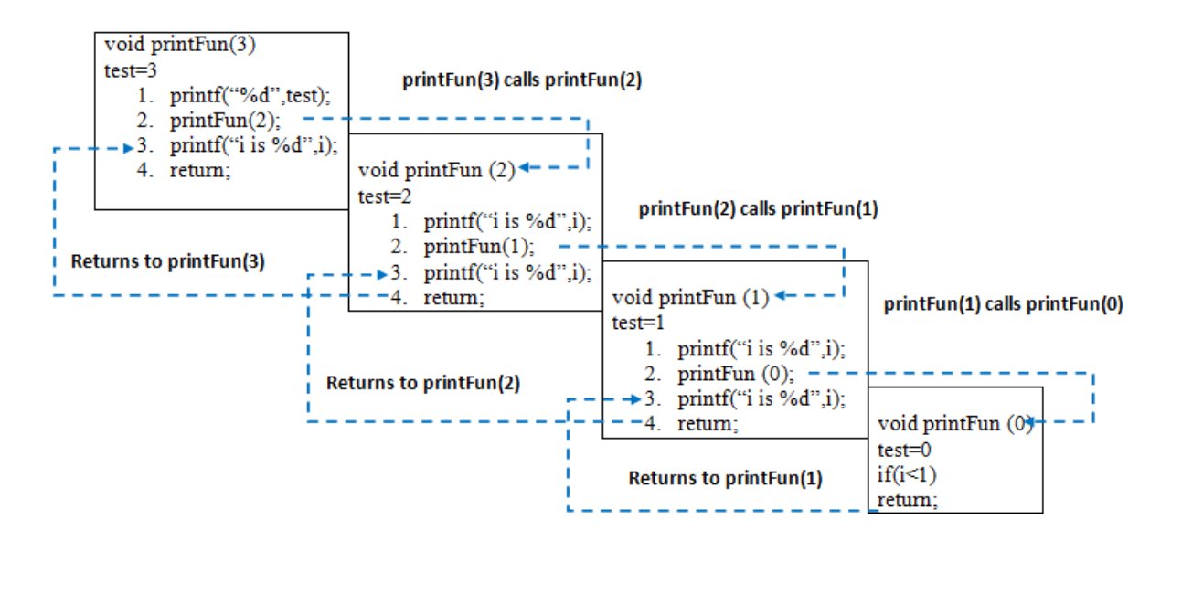
Let us take the example of how recursion works by taking a simple function.
Python3
def printFun(test):
if (test < 1):
return
else:
print(test, end=" ")
printFun(test-1)
print(test, end=" ")
return
test = 3
printFun(test)
|
The memory stack has been shown in below diagram.
More articles on Recursion
>>> More
Dynamic Programming
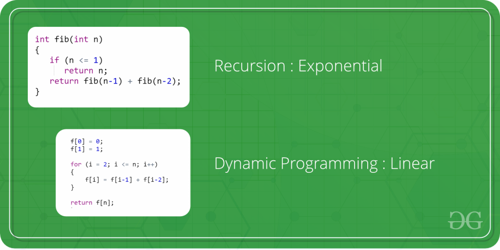
Dynamic Programming is mainly an optimization over plain recursion. Wherever we see a recursive solution that has repeated calls for same inputs, we can optimize it using Dynamic Programming. The idea is to simply store the results of subproblems, so that we do not have to re-compute them when needed later. This simple optimization reduces time complexities from exponential to polynomial. For example, if we write simple recursive solution for Fibonacci Numbers, we get exponential time complexity and if we optimize it by storing solutions of subproblems, time complexity reduces to linear.
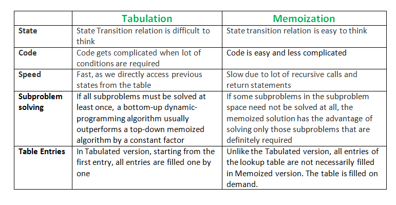
Tabulation vs Memoization
There are two different ways to store the values so that the values of a sub-problem can be reused. Here, will discuss two patterns of solving dynamic programming (DP) problem:
- Tabulation: Bottom Up
- Memoization: Top Down
Tabulation
As the name itself suggests starting from the bottom and accumulating answers to the top. Let’s discuss in terms of state transition.
Let’s describe a state for our DP problem to be dp[x] with dp[0] as base state and dp[n] as our destination state. So, we need to find the value of destination state i.e dp[n].
If we start our transition from our base state i.e dp[0] and follow our state transition relation to reach our destination state dp[n], we call it the Bottom-Up approach as it is quite clear that we started our transition from the bottom base state and reached the topmost desired state.
Now, Why do we call it tabulation method?
To know this let’s first write some code to calculate the factorial of a number using bottom up approach. Once, again as our general procedure to solve a DP we first define a state. In this case, we define a state as dp[x], where dp[x] is to find the factorial of x.
Now, it is quite obvious that dp[x+1] = dp[x] * (x+1)
# Tabulated version to find factorial x.
dp = [0]*MAXN

# base case
dp[0] = 1;
for i in range(n+1):
   dp[i] = dp[i-1] * i
Memoization
Once, again let’s describe it in terms of state transition. If we need to find the value for some state say dp[n] and instead of starting from the base state that i.e dp[0] we ask our answer from the states that can reach the destination state dp[n] following the state transition relation, then it is the top-down fashion of DP.
Here, we start our journey from the top most destination state and compute its answer by taking in count the values of states that can reach the destination state, till we reach the bottom-most base state.
Once again, let’s write the code for the factorial problem in the top-down fashion
# Memoized version to find factorial x.
#  To speed up we store the values
# of calculated states

# initialized to -1
dp[0]*MAXN

# return fact x!
def solve(x):
   if (x==0)
       return 1
   if (dp[x]!=-1)
       return dp[x]
   return (dp[x] = x * solve(x-1))
More articles on Dynamic Programming
>>> More
Searching Algorithms
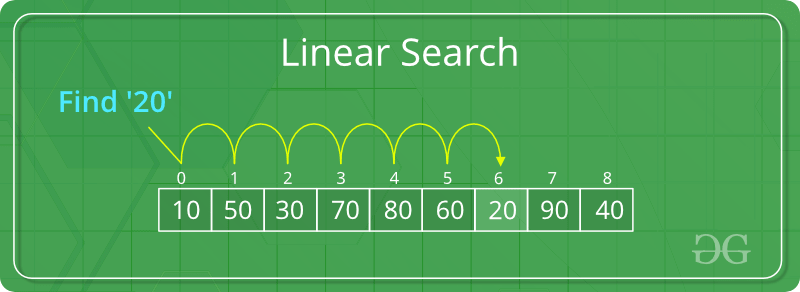
Linear Search
- Start from the leftmost element of arr[] and one by one compare x with each element of arr[]
- If x matches with an element, return the index.
- If x doesn’t match with any of the elements, return -1.
Python3
def search(arr, n, x):
for i in range(0, n):
if (arr[i] == x):
return i
return -1
arr = [2, 3, 4, 10, 40]
x = 10
n = len(arr)
result = search(arr, n, x)
if(result == -1):
print("Element is not present in array")
else:
print("Element is present at index", result)
|
Output
Element is present at index 3
The time complexity of the above algorithm is O(n).
For more information, refer to Linear Search.
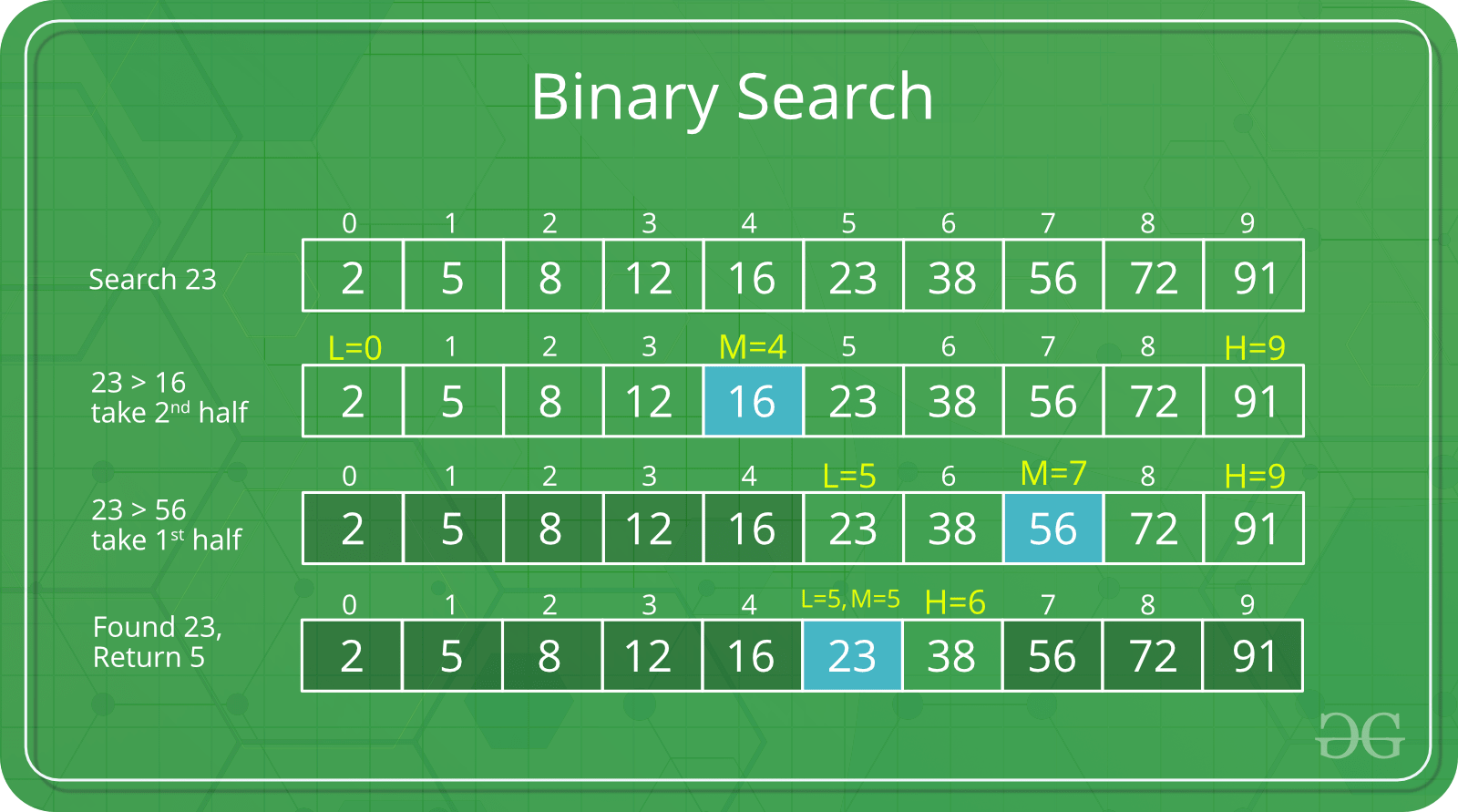
Binary Search
Search a sorted array by repeatedly dividing the search interval in half. Begin with an interval covering the whole array. If the value of the search key is less than the item in the middle of the interval, narrow the interval to the lower half. Otherwise, narrow it to the upper half. Repeatedly check until the value is found or the interval is empty.
Python3
def binarySearch (arr, l, r, x):
if r >= l:
mid = l + (r - l) // 2
if arr[mid] == x:
return mid
elif arr[mid] > x:
return binarySearch(arr, l, mid-1, x)
else:
return binarySearch(arr, mid + 1, r, x)
else:
return -1
arr = [ 2, 3, 4, 10, 40 ]
x = 10
result = binarySearch(arr, 0, len(arr)-1, x)
if result != -1:
print ("Element is present at index % d" % result)
else:
print ("Element is not present in array")
|
Output
Element is present at index 3
The time complexity of the above algorithm is O(log(n)).
For more information, refer to Binary Search.
Sorting Algorithms
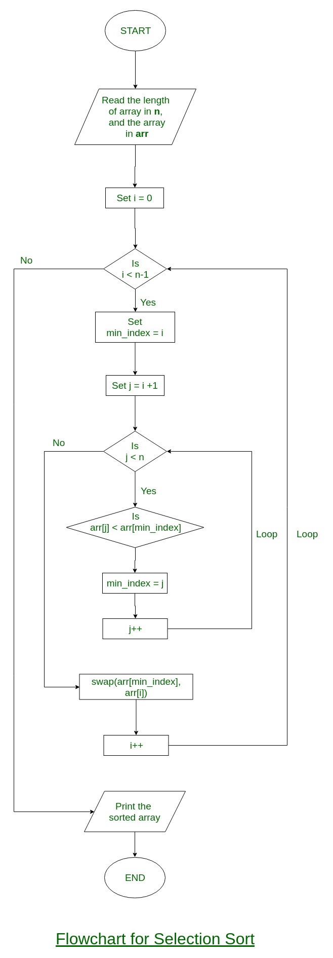
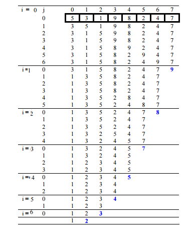
Selection Sort
The selection sort algorithm sorts an array by repeatedly finding the minimum element (considering ascending order) from unsorted part and putting it at the beginning. In every iteration of selection sort, the minimum element (considering ascending order) from the unsorted subarray is picked and moved to the sorted subarray.
Flowchart of the Selection Sort:
Python3
import sys
A = [64, 25, 12, 22, 11]
for i in range(len(A)):
min_idx = i
for j in range(i+1, len(A)):
if A[min_idx] > A[j]:
min_idx = j
A[i], A[min_idx] = A[min_idx], A[i]
print ("Sorted array")
for i in range(len(A)):
print("%d" %A[i]),
|
Output
Sorted array
11
12
22
25
64
Time Complexity: O(n2) as there are two nested loops.
Auxiliary Space: O(1)
Bubble Sort
Bubble Sort is the simplest sorting algorithm that works by repeatedly swapping the adjacent elements if they are in wrong order.
Illustration :
Python3
def bubbleSort(arr):
n = len(arr)
for i in range(n):
for j in range(0, n-i-1):
if arr[j] > arr[j+1] :
arr[j], arr[j+1] = arr[j+1], arr[j]
arr = [64, 34, 25, 12, 22, 11, 90]
bubbleSort(arr)
print ("Sorted array is:")
for i in range(len(arr)):
print ("%d" %arr[i]),
|
Output
Sorted array is:
11
12
22
25
34
64
90
Time Complexity: O(n2)
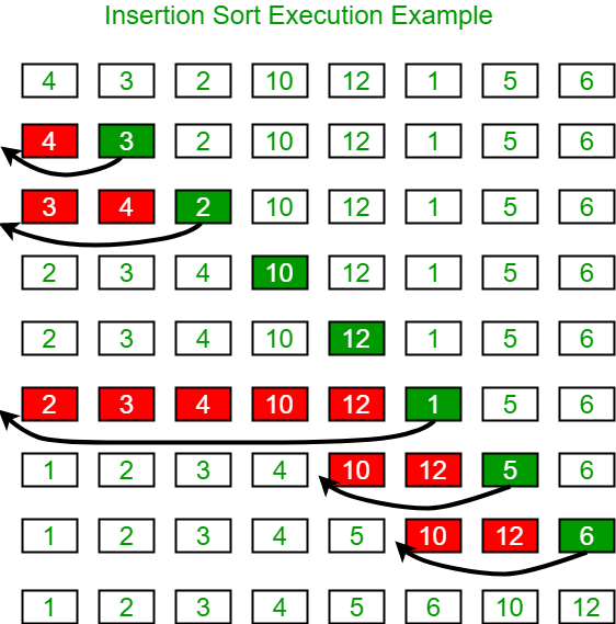
Insertion Sort
To sort an array of size n in ascending order using insertion sort:
- Iterate from arr[1] to arr[n] over the array.
- Compare the current element (key) to its predecessor.
- If the key element is smaller than its predecessor, compare it to the elements before. Move the greater elements one position up to make space for the swapped element.
Illustration:
Python3
def insertionSort(arr):
for i in range(1, len(arr)):
key = arr[i]
j = i-1
while j >= 0 and key < arr[j] :
arr[j + 1] = arr[j]
j -= 1
arr[j + 1] = key
arr = [12, 11, 13, 5, 6]
insertionSort(arr)
for i in range(len(arr)):
print ("% d" % arr[i])
|
Time Complexity: O(n2))
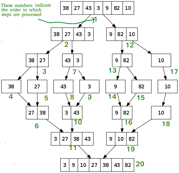
Merge Sort
Like QuickSort, Merge Sort is a Divide and Conquer algorithm. It divides the input array into two halves, calls itself for the two halves, and then merges the two sorted halves. The merge() function is used for merging two halves. The merge(arr, l, m, r) is a key process that assumes that arr[l..m] and arr[m+1..r] are sorted and merges the two sorted sub-arrays into one.
MergeSort(arr[], l,  r)
If r > l
     1. Find the middle point to divide the array into two halves:
             middle m = l+ (r-l)/2
     2. Call mergeSort for first half:
             Call mergeSort(arr, l, m)
     3. Call mergeSort for second half:
             Call mergeSort(arr, m+1, r)
     4. Merge the two halves sorted in step 2 and 3:
             Call merge(arr, l, m, r)
Python3
def mergeSort(arr):
if len(arr) > 1:
mid = len(arr)//2
L = arr[:mid]
R = arr[mid:]
mergeSort(L)
mergeSort(R)
i = j = k = 0
while i < len(L) and j < len(R):
if L[i] < R[j]:
arr[k] = L[i]
i += 1
else:
arr[k] = R[j]
j += 1
k += 1
while i < len(L):
arr[k] = L[i]
i += 1
k += 1
while j < len(R):
arr[k] = R[j]
j += 1
k += 1
def printList(arr):
for i in range(len(arr)):
print(arr[i], end=" ")
print()
if __name__ == '__main__':
arr = [12, 11, 13, 5, 6, 7]
print("Given array is", end="\n")
printList(arr)
mergeSort(arr)
print("Sorted array is: ", end="\n")
printList(arr)
|
Output
Given array is
12 11 13 5 6 7
Sorted array is:
5 6 7 11 12 13
Time Complexity: O(n(logn))
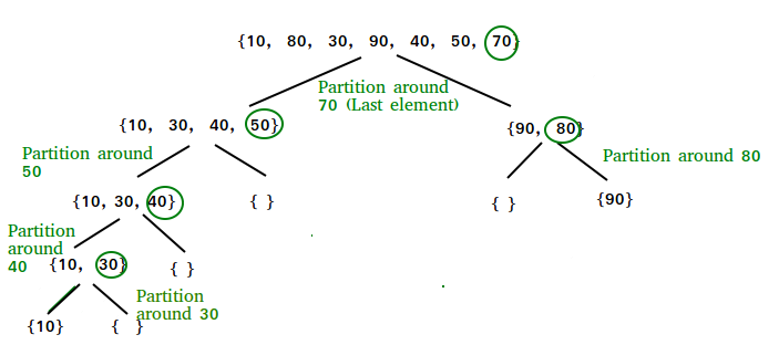
QuickSort
Like Merge Sort, QuickSort is a Divide and Conquer algorithm. It picks an element as pivot and partitions the given array around the picked pivot. There are many different versions of quickSort that pick pivot in different ways.
Always pick first element as pivot.
- Always pick last element as pivot (implemented below)
- Pick a random element as pivot.
- Pick median as pivot.
The key process in quickSort is partition(). Target of partitions is, given an array and an element x of array as pivot, put x at its correct position in sorted array and put all smaller elements (smaller than x) before x, and put all greater elements (greater than x) after x. All this should be done in linear time.
/* low  --> Starting index,  high  --> Ending index */
quickSort(arr[], low, high)
{
    if (low < high)
    {
        /* pi is partitioning index, arr[pi] is now
           at right place */
        pi = partition(arr, low, high);

        quickSort(arr, low, pi - 1);  // Before pi
        quickSort(arr, pi + 1, high); // After pi
    }
}
Partition Algorithm
There can be many ways to do partition, following pseudo code adopts the method given in CLRS book. The logic is simple, we start from the leftmost element and keep track of index of smaller (or equal to) elements as i. While traversing, if we find a smaller element, we swap current element with arr[i]. Otherwise we ignore current element.
/* This function takes last element as pivot, places the pivot element at its correct position in sorted array, and places all smaller (smaller than pivot) to left of pivot and all greater elements to right of pivot */

partition (arr[], low, high)
{
    // pivot (Element to be placed at right position)
    pivot = arr[high];

    i = (low – 1)  // Index of smaller element and indicates the
    // right position of pivot found so far

    for (j = low; j <= high- 1; j++){

        // If current element is smaller than the pivot
        if (arr[j] < pivot){
            i++;    // increment index of smaller element
            swap arr[i] and arr[j]
        }
    }
    swap arr[i + 1] and arr[high])
    return (i + 1)
}
Python3
def partition(start, end, array):
pivot_index = start
pivot = array[pivot_index]
while start < end:
while start < len(array) and array[start] <= pivot:
start += 1
while array[end] > pivot:
end -= 1
if(start < end):
array[start], array[end] = array[end], array[start]
array[end], array[pivot_index] = array[pivot_index], array[end]
return end
def quick_sort(start, end, array):
if (start < end):
p = partition(start, end, array)
quick_sort(start, p - 1, array)
quick_sort(p + 1, end, array)
array = [ 10, 7, 8, 9, 1, 5 ]
quick_sort(0, len(array) - 1, array)
print(f'Sorted array: {array}')
|
Output
Sorted array: [1, 5, 7, 8, 9, 10]
Time Complexity: O(n(logn))
ShellSort
ShellSort is mainly a variation of Insertion Sort. In insertion sort, we move elements only one position ahead. When an element has to be moved far ahead, many movements are involved. The idea of shellSort is to allow the exchange of far items. In shellSort, we make the array h-sorted for a large value of h. We keep reducing the value of h until it becomes 1. An array is said to be h-sorted if all sublists of every hth element is sorted.
Python3
def shellSort(arr):
gap = len(arr) // 2
while gap > 0:
i = 0
j = gap
while j < len(arr):
if arr[i] >arr[j]:
arr[i],arr[j] = arr[j],arr[i]
i += 1
j += 1
k = i
while k - gap > -1:
if arr[k - gap] > arr[k]:
arr[k-gap],arr[k] = arr[k],arr[k-gap]
k -= 1
gap //= 2
arr2 = [12, 34, 54, 2, 3]
print("input array:",arr2)
shellSort(arr2)
print("sorted array",arr2)
|
Output
input array: [12, 34, 54, 2, 3]
sorted array [2, 3, 12, 34, 54]
Time Complexity: O(n2).
Like Article
Suggest improvement
Share your thoughts in the comments
Please Login to comment...