Python language is one of the most trending programming languages as it is dynamic than others. Python is a simple high-level and an open-source language used for general-purpose programming. It has many open-source libraries and Pandas is one of them. Pandas is a powerful, fast, flexible open-source library used for data analysis and manipulations of data frames/datasets. Pandas can be used to read and write data in a dataset of different formats like CSV(comma separated values), txt, xls(Microsoft Excel) etc.
In this post, you will learn about various features of Pandas in Python and how to use it to practice.
Prerequisites: Basic knowledge about coding in Python.
Installation:
So if you are new to practice Pandas, then firstly you should install Pandas on your system.
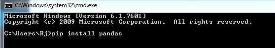
Go to Command Prompt and run it as administrator. Make sure you are connected with an internet connection to download and install it on your system.
Then type “pip install pandas“, then press Enter key.
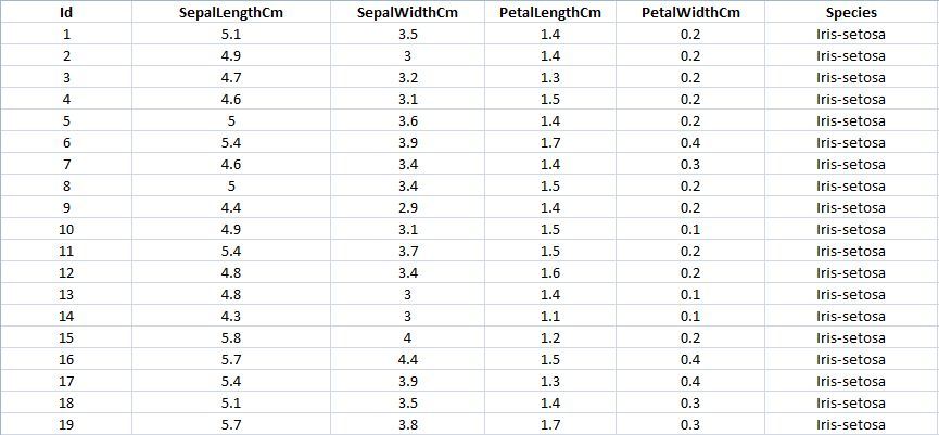
Download the Dataset “Iris.csv”.
Iris dataset is the Hello World for the Data Science, so if you have started your career in Data Science and Machine Learning you will be practicing basic ML algorithms on this famous dataset. Iris dataset contains five columns such as Petal Length, Petal Width, Sepal Length, Sepal Width and Species Type.
Iris is a flowering plant, the researchers have measured various features of the different iris flowers and recorded digitally.
Getting Started with Pandas:
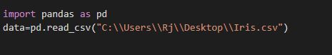
Code: Importing pandas to use in our code as pd.
Code: Reading the dataset “Iris.csv”.
Python3
data = pd.read_csv("your downloaded dataset location ")
|
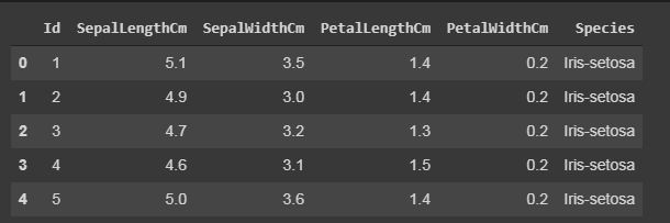
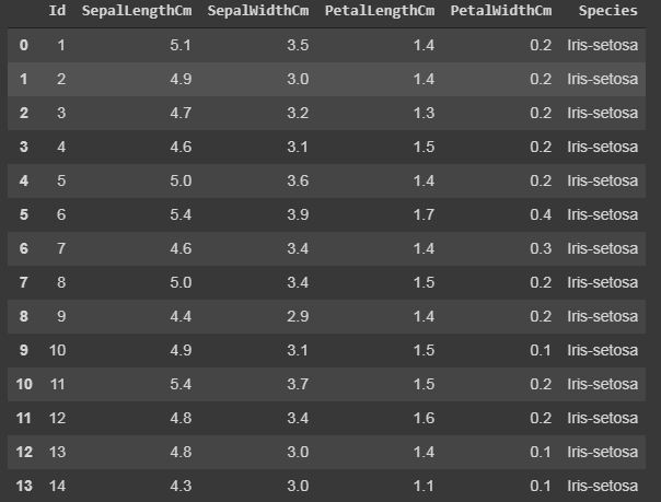
Code: Displaying up the top rows of the dataset with their columns
The function head() will display the top rows of the dataset, the default value of this function is 5, that is it will show top 5 rows when no argument is given to it.
Output:
Displaying the number of rows randomly.
In sample() function, it will also display the rows according to arguments given, but it will display the rows randomly.
Output:

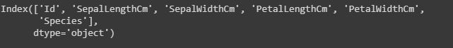
Code: Displaying the number of columns and names of the columns.
The column() function prints all the columns of the dataset in a list form.
Output:
Code: Displaying the shape of the dataset.
The shape of the dataset means to print the total number of rows or entries and the total number of columns or features of that particular dataset.
Output:

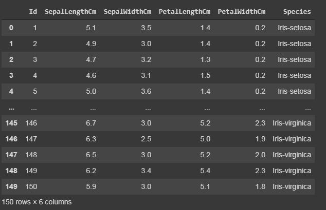
Code: Display the whole dataset
Output:
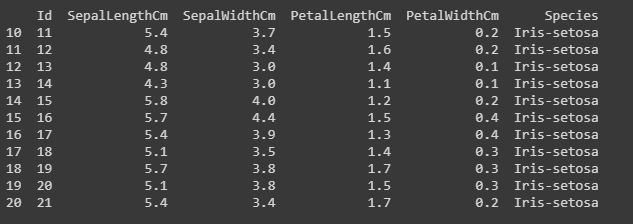
Code: Slicing the rows.
Slicing means if you want to print or work upon a particular group of lines that is from 10th row to 20th row.
Python3
print(data[10:21])
sliced_data=data[10:21]
print(sliced_data)
|
Output:
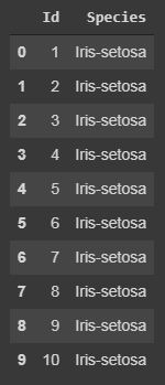
Code: Displaying only specific columns.
In any dataset, it is sometimes needed to work upon only specific features or columns, so we can do this by the following code.
Python3
specific_data=data[["Id","Species"]]
print(specific_data.head(10))
|
Output:
Filtering:Displaying the specific rows using “iloc” and “loc” functions.
The “loc” functions use the index name of the row to display the particular row of the dataset.
The “iloc” functions use the index integer of the row, which gives complete information about the row.
Code:
Python3
data.iloc[5]
data.loc[data["Species"] == "Iris-setosa"]
|
Output:
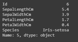
iloc()[/caption]
loc()
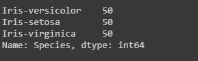
Code: Counting the number of counts of unique values using “value_counts()”.
The value_counts() function, counts the number of times a particular instance or data has occurred.
Python3
data["Species"].value_counts()
|
Output:
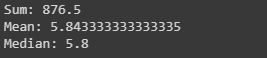
Calculating sum, mean and mode of a particular column.
We can also calculate the sum, mean and mode of any integer columns as I have done in the following code.
Python3
sum_data = data["SepalLengthCm"].sum()
mean_data = data["SepalLengthCm"].mean()
median_data = data["SepalLengthCm"].median()
print("Sum:",sum_data, "\nMean:", mean_data, "\nMedian:",median_data)
|
Output:
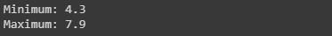
Code: Extracting minimum and maximum from a column.
Identifying minimum and maximum integer, from a particular column or row can also be done in a dataset.
Python3
min_data=data["SepalLengthCm"].min()
max_data=data["SepalLengthCm"].max()
print("Minimum:",min_data, "\nMaximum:", max_data)
|
Output:
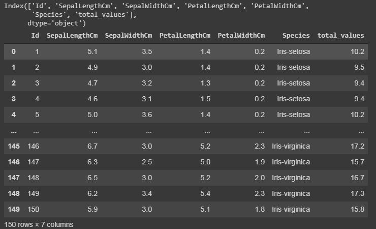
Code: Adding a column to the dataset.
If want to add a new column in our dataset, as we are doing any calculations or extracting some information from the dataset, and if you want to save it a new column. This can be done by the following code by taking a case where we have added all integer values of all columns.
Python3
cols = data.columns
print(cols)
cols = cols[1:5]
data1 = data[cols]
data["total_values"]=data1[cols].sum(axis=1)
|
Output:
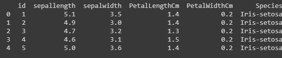
Code: Renaming the columns.
Renaming our column names can also be possible in python pandas libraries. We have used the rename() function, where we have created a dictionary “newcols” to update our new column names. The following code illustrates that.
Python3
newcols={
"Id":"id",
"SepalLengthCm":"sepallength"
"SepalWidthCm":"sepalwidth"}
data.rename(columns=newcols,inplace=True)
print(data.head())
|
Output:
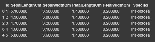
Formatting and Styling:
Conditional formatting can be applied to your dataframe by using Dataframe.style function. Styling is used to visualize your data, and most convenient way of visualizing your dataset is in tabular form.
Here we will highlight the minimum and maximum from each row and columns.
Python3
which is not visualised by any styles.
data.style
|
Output:
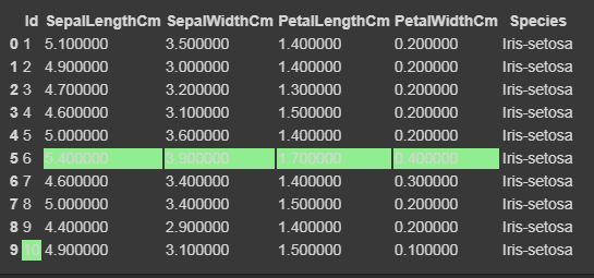
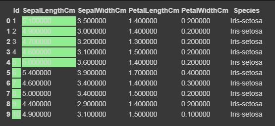
Now we will highlight the maximum and minimum column-wise, row-wise, and the whole dataframe wise using Styler.apply function. The Styler.apply function passes each column or row of the dataframe depending upon the keyword argument axis. For column-wise use axis=0, row-wise use axis=1, and for the entire table at once use axis=None.
Python3
data.head(10).style.highlight_max(color='lightgreen', axis=0)
data.head(10).style.highlight_max(color='lightgreen', axis=1)
data.head(10).style.highlight_max(color='lightgreen', axis=None)
|
Output:
for axis=0
for axis=1
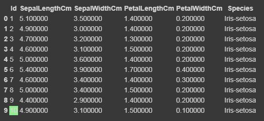
for axis=None
Code: Cleaning and detecting missing values
In this dataset, we will now try to find the missing values i.e NaN, which can occur due to several reasons.
Output:
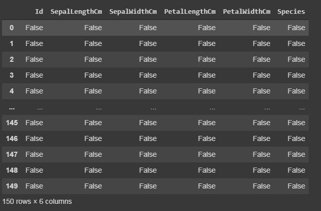
isnull()
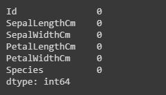
Code: Summarizing the missing values.
We will display how many missing values are present in each column.
Output:
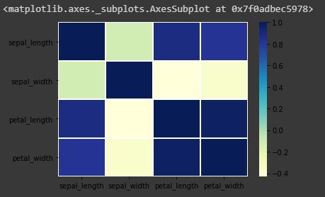
Heatmap: Importing seaborn
The heatmap is a data visualisation technique which is used to analyse the dataset as colors in two dimensions. Basically it shows correlation between all numerical variables in the dataset. Heatmap is an attribute of the Seaborn library.
Code:
Python3
import seaborn as sns
iris = sns.load_dataset("iris")
sns.heatmap(iris.corr(),camp = "YlGnBu", linecolor = 'white', linewidths = 1)
|
Output:
Code: Annotate each cell with the numeric value using integer formatting
Python3
sns.heatmap(iris.corr(),camp = "YlGnBu", linecolor = 'white', linewidths = 1, annot = True )
|
Output:
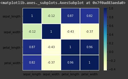
heatmap with annot=True
Pandas Dataframe Correlation:
Pandas correlation is used to determine pairwise correlation of all the columns of the dataset. In dataframe.corr(), the missing values are excluded and non-numeric columns are also ignored.
Code:
Python3
data.corr(method='pearson')
|
Output:
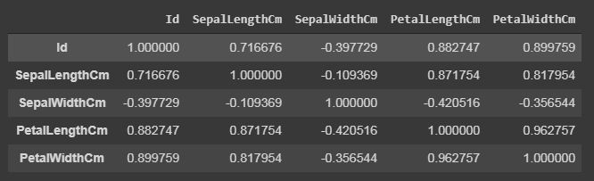
data.corr()
The output dataframe can be seen as for any cell, row variable correlation with the column variable is the value of the cell. The correlation of a variable with itself is 1. For that reason, all the diagonal values are 1.00.
Multivariate Analysis:
Pair plot is used to visualize the relationship between each type of column variable. It is implemented only by one line code, which is as follows :
Code:
Python3
g = sns.pairplot(data,hue="Species")
|
Output:
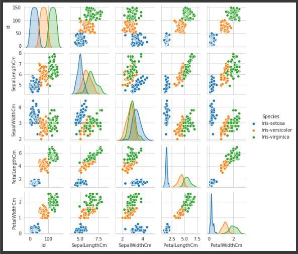
Pairplot of variable “Species”, to make it more understandable.
Share your thoughts in the comments
Please Login to comment...