Processing of Raw Data to Tidy Data in R

The data that is download from web or other resources are often hard to analyze. It is often needed to do some processing or cleaning of the dataset in order to prepare it for further downstream analysis, predictive modeling and so on. This article discusses several methods in R to convert the raw dataset into a tidy data.

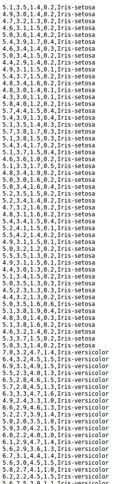
Raw Data

A Raw data is a dataset that has been downloaded from web (or any other source) and has not been processed yet. Raw data is not ready for use in statistics. It needs various processing tools to be ready for analysis.

Example: Below is the image of a Raw IRIS Dataset. It does not have any information as what the data is, or what is it representing. This will be done by tidying the data.

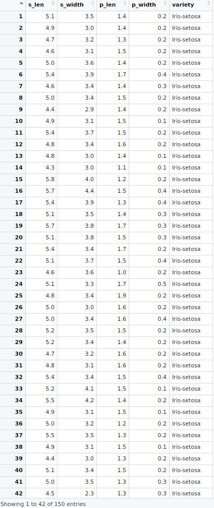
Tidy Data

On the other hand, a Tidy dataset (also called cooked data) is the data that has following characteristics:

• Each variable measured should be in one column.
• Each different observation of that variable should be in a different row.
• There should be one table for each “kind” of variable.
• If there are multiple tables, they should include a column in the table that allows them to be linked.

Example: Below is the image of a Tidy IRIS Dataset. It contains valuable processed information like column names. The process is explained later below.

Steps in general processing a raw dataset into a tidy dataset with example

1. Loading the dataset in R
   • The first-most step is to get the data for processing. Here the data taken is from IRIS data.
   • Firstly download the data and make it into a dataframe in R.

     ##Provide the link of the dataset
     url < -"http:// archive.ics.uci.edu/ml/machine-learning-databases/iris/iris.data"
     
     ##download the data in a file iris.txt
     ##will be saved in the working directory
     download.file(url, "iris.txt")
     
     ##import the data in a dataframe
     d < -read.table("iris.txt", sep = ", ")
     
     ##Rename the columns
     colnames(d)< -c("s_len",
              "s_width",
              "p_len",
              "p_width",
              "variety")
2. Subsetting Rows and Columns
   • Now if only s_len(1st column), p_len(3rd column) and variety(5th column) are required for analysis, then subset these columns and assign the new data to a new dataframe.

     ##subsetting columns with column number
     d1 <- d[, c(1, 3, 5)]
   • Subsetting can also be done using column names.

     ##subsetting columns with column names
     d1 <- d[, c("s_len", "p_len", "variety")]
   • Also, If it is required to know the observations that are either of variety “Iris-setosa” or have “sepal length less than 5”.

     ##Subsetting the rows
     d2 <- d[(d$s_len < 5 | d$variety == "Iris-setosa"), ]

   Note: The “$” operator is used to subset a column.

3. Sorting the data frame by some variable

   Order the dataframe by petal length using the order command.

   d3 < -d[order(d$p_len), ]
4. Adding new rows and columns

   Add a new column by cbind() and add new row by rbind().

   ##Extract the s_width column of d
   sepal_width <- d$s_width
   
   ##Add the column to d1 dataframe.
   d1 <- cbind(d1, sepal_width)
5. Getting an overview of the data at a glance
   • To get a summarised overview of the processed data, call summary() command on the data-frame.

     summary(d)

     Output“:

        s_len          s_width          p_len          p_width                 variety  
      Min.   :4.300   Min.   :2.000   Min.   :1.000   Min.   :0.100   Iris-setosa    :50  
      1st Qu.:5.100   1st Qu.:2.800   1st Qu.:1.600   1st Qu.:0.300   Iris-versicolor:50  
      Median :5.800   Median :3.000   Median :4.350   Median :1.300   Iris-virginica :50  
      Mean   :5.843   Mean   :3.054   Mean   :3.759   Mean   :1.199                       
      3rd Qu.:6.400   3rd Qu.:3.300   3rd Qu.:5.100   3rd Qu.:1.800                       
      Max.   :7.900   Max.   :4.400   Max.   :6.900   Max.   :2.500                       
     

   • To get overview like the type of each variable, total number of observations, and their first few values; use str() command.

     str(d)

     Output:

     'data.frame':    150 obs. of  5 variables:
      $ s_len  : num  5.1 4.9 4.7 4.6 5 5.4 4.6 5 4.4 4.9 ...
      $ s_width: num  3.5 3 3.2 3.1 3.6 3.9 3.4 3.4 2.9 3.1 ...
      $ p_len  : num  1.4 1.4 1.3 1.5 1.4 1.7 1.4 1.5 1.4 1.5 ...
      $ p_width: num  0.2 0.2 0.2 0.2 0.2 0.4 0.3 0.2 0.2 0.1 ...
      $ variety: Factor w/ 3 levels "Iris-setosa", ..: 1 1 1 1 1 1 1 1 1 1 ...
     

Reshaping the data using Melt() and Cast()

• Another way of re-organizing data is by using melt and cast functions. They are present in reshape2 package.

  ## Create A Dummy Dataset
  d<-data.frame(
       name=c("Arnab", "Arnab", "Soumik", "Mukul", "Soumik"),
       year=c(2011, 2014, 2011, 2015, 2014),
       height=c(5, 6, 4, 3, 5),
       Weight=c(90, 89, 76, 85, 84))
  
  ## View the dataset
  d

  Output:

      name year height Weight
  1  Arnab 2011      5     90
  2  Arnab 2014      6     89
  3 Soumik 2011      4     76
  4  Mukul 2015      3     85
  5 Soumik 2014      5     84
  

• Melting of this data means referring some variable as id variable (Others will be taken as measure variables). Now if name and year are taken as id variable and height and weight as measure variables, then there will be 4 columns in the new dataset- name, year, variable and value. For each name and year, there will be the variable to be measured and its value.

  ## Getting the reshape library
  install.packages("reshape2")
  library(reshape2)
  
  ## Configure the id variables, name and year
  melt(d, id=c("name", "year"))

  Output:

       name year variable value
  1   Arnab 2011   height     5
  2   Arnab 2014   height     6
  3  Soumik 2011   height     4
  4   Mukul 2015   height     3
  5  Soumik 2014   height     5
  6   Arnab 2011   Weight    90
  7   Aranb 2014   Weight    89
  8  Soumik 2011   Weight    76
  9   Mukul 2015   Weight    85
  10 Soumik 2014   Weight    84
  

• Now the molten dataset can be converted in a compact form by cast() function. Compute everyone’s mean height and weight.

  ##Save the molten dataset
  d1<-melt(d, id=c("name", "year"))
  
  ##Now cast the data
  d2 <-cast(d1, name~variable, mean)
  
  ## View the data
  d2

  Output:

  name height Weight
  1  Arnab    5.5   89.5
  2  Mukul    3.0   85.0
  3 Soumik    4.5   80.0
  

Note: There are also some other packages like dplyr and tidyr in R that provide functions for preparing tidy data.