Polynomial Regression using Turicreate
Last Updated :
24 Jan, 2021
In this article, we will discuss the implementation of Polynomial Regression using Turicreate. Polynomial Regression: Polynomial regression is a form of regression analysis that models the relationship between a dependent say y and an independent variable say x as a nth degree polynomial. It is expressed as :
y= b0+b1x1+ b2x12+ b2x13+…… bnx1n
[where b0, b1, b2, …… bn are regression coefficients]
So let’s learn this concept through practicals.
Step 1: Import the important libraries and generate a very small data set using SArray and SFrame in turicreate that we are going to use to perform Polynomial Regression.
Python3
import turicreate
import matplotlib.pyplot as plt
import random
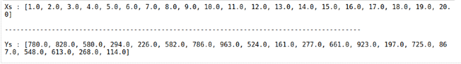
X = [data for data in range(1, 21)]
Y = [random.randrange(100, 1000, 1) for data in range(20)]
Xs = turicreate.SArray(X, dtype=float)
Ys = turicreate.SArray(Y, dtype=float)
print(f
)
|
Output:
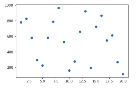
Step 2: Plotting the generated data
Python3
plt.scatter(Xs, Ys)
plt.show()
|
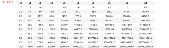
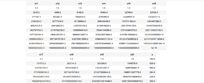
Step 3: Create an SFrame containing the input, its polynomial_degrees, and the output in order to fit our regression model.
Python3
def createSframe(inputs, pol_degree):
datapoints = turicreate.SFrame({'x1': inputs})
for degree in range(2, pol_degree+1):
datapoints[f'x{degree}'] = datapoints[f'x{degree-1}']*datapoints['x1']
return datapoints
data_points = createSframe(Xs, 20)
data_points['y'] = Ys
data_points.head()
|
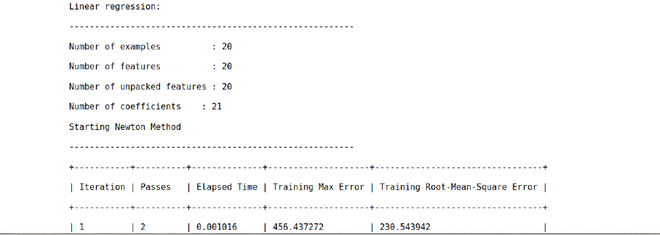
Step 4: Fitting Polynomial Regression to the generated Data set.
Python3
features = [f'x{i}' for i in range(1, 21)]
poly_model = turicreate.linear_regression.create(
data_points, features=features, target='y')
|
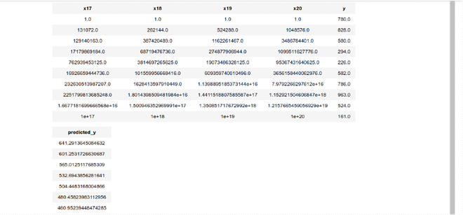
Step 5: Predicting the result using the fitted model and storing the result in the SFrame.
Python3
test_X = [random.randrange(1, 60, 1) for data in range(20)]
test_Xs = turicreate.SArray(X, dtype=float)
test_data = createSframe(test_Xs, 5)
data_points['predicted_y'] = poly_model.predict(test_data)
data_points.head()
|
Step 6: Measuring the accuracy of our predicted result
Python
test_X = [random.randrange(1, 60, 1) for data in range(20)]
test_Xs = turicreate.SArray(X, dtype=float)
test_data = createSframe(test_Xs, 20)
poly_model.evaluate(data_points)
|

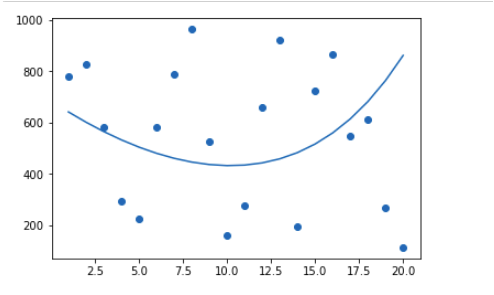
Step 7: Visualizing the Polynomial Regression results using scatter plot and line plot of the input data and the predicted result.
Python3
plt.scatter(data_points['x1'], data_points['y'])
plt.plot(data_points['x1'], data_points['predicted_y'])
plt.show()
|
Like Article
Suggest improvement
Share your thoughts in the comments
Please Login to comment...