Polynomial Regression in Julia

In statistics, polynomial regression is a form of regression analysis in which the relationship between the independent variable x and the dependent variable y is modeled as an nth degree polynomial in x. Polynomial regression fits a nonlinear relationship between the value of x and the corresponding conditional mean of y, denoted E(y |x). Polynomial regression is one example of regression analysis using basis functions to model a functional relationship between two quantities.

Advantages of Polynomial regression over linear regression

• Polynomial provides the best approximation of the relationship between the dependent and independent variables.
• A broad range of functions can be fit under it.
• Polynomial basically fits a wide range of curvature.

Polynomial Regression in Julia

Polynomial Regression in Julia can be implemented by using Polynomials.jl package. Polynomials.jl is a Julia package that provides basic arithmetic, integration, differentiation, evaluation, and root finding over dense univariate polynomials.

To install the package, run

pkg> add Polynomials

Once the package installed, you can load the package using

using Polynomials

Types of Polynomials

• Polynomial: Standard basis polynomials, a(x) = a₀ + a₁ x + a₂ x² + … + aₙ xⁿ, n ∈ ℕ
• ImmutablePolynomial: Standard basis polynomials backed by a Tuple type for faster evaluation of values
• SparsePolynomial:⁠ Standard basis polynomial backed by a dictionary to hold sparse high-degree polynomials
• LaurentPolynomial:⁠ Laurent polynomials, a(x) = aₘ xᵐ + … + aₙ xⁿ m ≤ n, m,n ∈ ℤ backed by an offset array; for example, if m<0 and n>0, a(x) = aₘ xᵐ + … + a₋₁ x⁻¹ + a₀ + a₁ x + … + aₙ xⁿ
• ChebyshevT:⁠ Chebyshev polynomials of the first kind

Syntax:

julia> using Polynomials

Now, let’s see how can we use Polynomial.jl to achieve arithmetic, integration, differentiation, evaluation, and root finding over dense univariate polynomials.

Construction and Evaluation

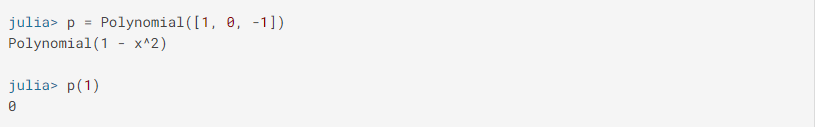
• Construct a polynomial from an array of its coefficients, lowest order first.

• Construct a polynomial from its roots by entering the roots as the parameters of the function of function fromroots() in the form of an array

• Evaluate the polynomial p at x by entering the coefficients as the parameters of function polynomial() in the form of an array

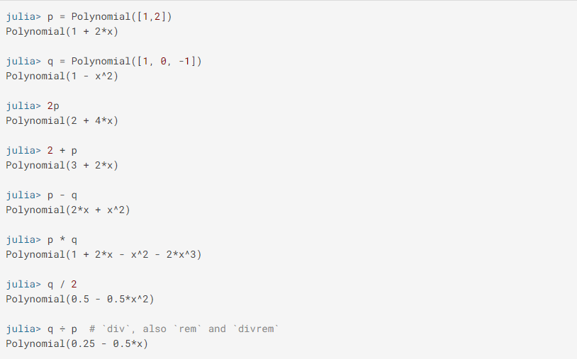
Arithmetic Operators on Polynomials

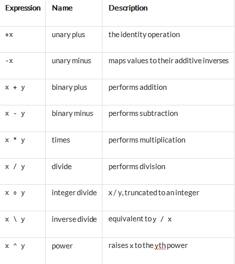
The usual arithmetic operators are overloaded to work on polynomials and combinations of polynomials and scalars.

The following arithmetic operators are supported on all primitive numeric types:

Integrals and Derivatives

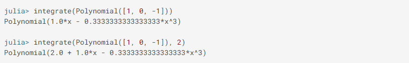
Integrate the polynomial p term by term, optionally adding a constant term k. The degree of the resulting polynomial is one higher than the degree of p (for a nonzero polynomial).

Differentiate the polynomial p term by term. The degree of the resulting polynomial is one lower than the degree of p.

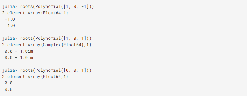
Finding Roots of Polynomials

Return the roots (zeros) of p, with multiplicity. The number of roots returned is equal to the degree of p. By design, this is not type-stable, the returned roots may be real or complex.

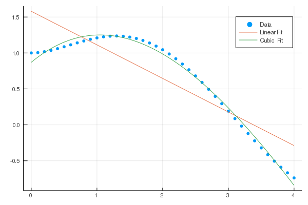
Fitting Arbitrary Data

Fit a polynomial (of degree deg or less) to x and y using a least-squares approximation.

Julia

using Plots, Polynomials
xs = range(0, 10, length = 10)
ys = @.exp(-xs)
f = fit(xs, ys) # degree = length(xs) - 1
f2 = fit(xs, ys, 2) # degree = 2

scatter(xs, ys, markerstrokewidth = 0, label = "Data")
plot!(f, extrema(xs)..., label = "Fit")
plot!(f2, extrema(xs)..., label = "Quadratic Fit")