Plot t Distribution in R

The t-distribution, also known as the Student’s t-distribution is a type of probability distribution that is used to perform sampling of a normally distributed distribution where the sample size is small and the standard deviation of the input distribution is unknown. The distribution normally forms a bell curve, that is, the distribution is normally distributed but with a lower peak and more observations near the tail. 

The t-distribution has only one associated parameter, called the degrees of freedom (df). The shape of a particular t-distribution curve relies on the number of degrees of freedom (df) chosen which is equivalent to the given sample size minus one, that is,

df=n−1

A vector of coordinates can be generated using the seq() method in R, which is used to generate an incremental sequence of integers to provide a distribution sequence for the given t-distribution. The corresponding y coordinates can be constructed using the various variants of the t-distribution function which are detailed below. These are then plotted using the plot() method in R programming language.

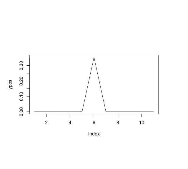
dt() method

The dt() method in R is used to compute probability density analysis of the t-distribution with a specified degree of freedom. 

Syntax:

dt(x, df )

Parameter : 

• x – vector of quantiles
• df – degrees of freedom

Example:

R

# generating x coordinates
xpos <- seq(- 100, 100, by = 20)

print ("X coordinates")
print (xpos)

# generating y coordinates using dt() method
# degreesoffreedom
degree <- 2
ypos <- dt(xpos, df = degree)

print ("Y coordinates")
print (ypos)

# plotting t distribution
plot (ypos , type = "l")

Output

[1] “X coordinates” 

[1] -100  -80  -60  -40  -20    0   20   40   60   80  100

[1] “Y coordinates” 

[1] 9.997001e-07 1.952210e-06 4.625774e-06 1.559575e-05 1.240683e-04  [6] 3.535534e-01 1.240683e-04 1.559575e-05 4.625774e-06 1.952210e-06 

[11] 9.997001e-07

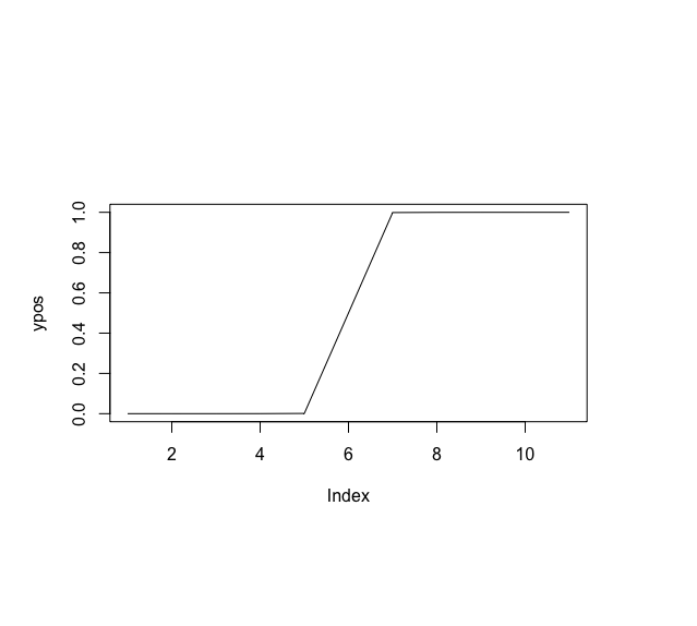
pt() method

The pt() method in R is used to produce a distribution function for a given student T-distribution. It is used to produce a cumulative distribution function. This function returns the area under the t-curve for any given interval. 

Syntax:

pt(q, df, lower.tail = TRUE)

Parameter : 

• q – quantile vector
• df – degrees of freedom
• lower.tail – if TRUE (default), probabilities are P[X ≤ x], otherwise, P[X > x].

Example:

R

# generating x coordinates
xpos <- seq(- 100, 100, by = 20)

print ("X coordinates")
print (xpos)

# generating y coordinates using dt() method
# degreesoffreedom
degree <- 2

ypos <- pt(xpos, df = degree)

print ("Y coordinates")
print (ypos)

# plotting t distribution
plot (ypos , type = "l")

Output

[1] “X coordinates” 

[1] -100  -80  -60  -40  -20    0   20   40   60   80  100 

[1] “Y coordinates” 

[1] 4.999250e-05 7.810669e-05 1.388310e-04 3.122073e-04 1.245332e-03  [6] 5.000000e-01 9.987547e-01 9.996878e-01 9.998612e-01 9.999219e-01 

[11] 9.999500e-01

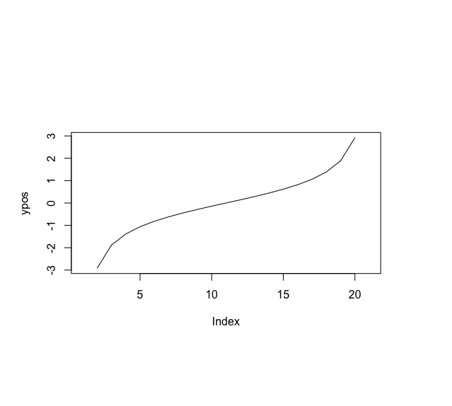
qt() method

The qt() method in R is used to compute a quantile function or inverse cumulative density function for the given t-distribution for a specified number of degrees of freedom. It is used to compute the nth percentile of the student’s t-distribution with a specified degree of freedom.  

Syntax:

qt(p, df, lower.tail = TRUE)

Parameter : 

• p – vector of probabilities
• df – degrees of freedom
• lower.tail – if TRUE (default), probabilities are P[X ≤ x], otherwise, P[X > x].

Example:

R

# generating x coordinates
xpos <- seq(0, 1, by = 0.05)

# generating y coordinates using dt() method
# degreesoffreedom
degree <- 2
ypos <- qt(xpos, df = degree)

# plotting t distribution
plot (ypos , type = "l")

Output

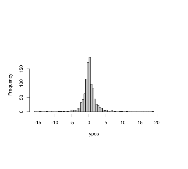
rt() method

The rt() method is used for random generation for the t distribution using a specified number of degrees of freedom. n number of random samples may be generated.

Syntax:

rt(n, df)

Parameter : 

• n – number of observations
• df – degrees of freedom

Example:

R

# using a random number
n <- 1000

# degreesoffreedom
degree <- 2

# generating y coordinates using rt() method
ypos <- rt(n , df = degree)

# plotting t distribution in the form of
# distribution
hist(ypos,
     breaks = 100,
     main = "")

Output