Parkinson Disease Prediction using Machine Learning – Python

Parkinson’s disease is a progressive disorder that affects the nervous system and the parts of the body controlled by the nerves. Symptoms are also not that sound to be noticeable. Signs of stiffening, tremors, and slowing of movements may be signs of Parkinson’s disease.

But there is no ascertain way to tell whether a person has Parkinson’s disease or not because there are no such diagnostics methods available to diagnose this disorder. But what if we use machine learning to predict whether a person suffers from Parkinson’s disease or not? This is exactly what we’ll be learning in this article.

Parkinson Disease Prediction using Machine Learning in Python

Importing Libraries and Dataset

Python libraries make it very easy for us to handle the data and perform typical and complex tasks with a single line of code.

• Pandas – This library helps to load the data frame in a 2D array format and has multiple functions to perform analysis tasks in one go.
• Numpy – Numpy arrays are very fast and can perform large computations in a very short time.
• Matplotlib/Seaborn – This library is used to draw visualizations.
• Sklearn – This module contains multiple libraries having pre-implemented functions to perform tasks from data preprocessing to model development and evaluation.
• XGBoost – This contains the eXtreme Gradient Boosting machine learning algorithm which is one of the algorithms which helps us to achieve high accuracy on predictions.
• Imblearn – This module contains a function that can be used for handling problems related to data imbalance.

Python3

import numpy as np
import pandas as pd
import matplotlib.pyplot as plt
import seaborn as sb

from imblearn.over_sampling import RandomOverSampler
from sklearn.model_selection import train_test_split
from sklearn.preprocessing import LabelEncoder, MinMaxScaler
from sklearn.feature_selection import SelectKBest, chi2
from tqdm.notebook import tqdm
from sklearn import metrics
from sklearn.svm import SVC
from xgboost import XGBClassifier
from sklearn.linear_model import LogisticRegression

import warnings
warnings.filterwarnings('ignore')

The dataset we are going to use here includes 755 columns and three observations for each patient. The value’s in these columns are part of some other diagnostics which are generally used to capture the difference between a healthy and affected person. Now, let’s load the dataset into the panda’s data frame.

Python3

df = pd.read_csv('parkinson_disease.csv')

Now let’s check the size of the dataset.

Python3

df.shape

Output:

 (756, 755)

The dataset is very high dimensional as the feature space contains 755 columns. Let’s check which column of the dataset contains which type of data.

Python3

df.info()

Output:

Information regarding data in the columns

As per the above information regarding the data in each column we can observe that there are no null values.

Python3

df.describe()

Output:

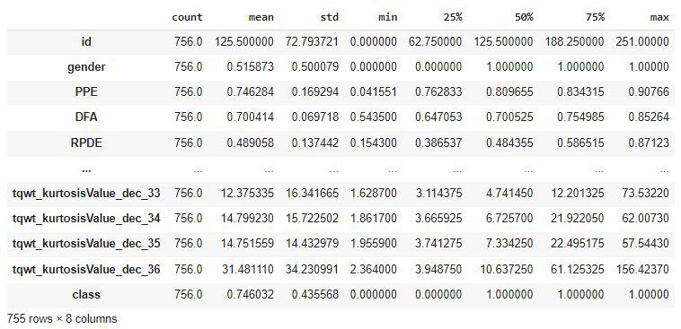
Descriptive statistical measures of the dataset

Data Cleaning

The data which is obtained from the primary sources is termed the raw data and required a lot of preprocessing before we can derive any conclusions from it or to some modeling on it. Those preprocessing steps are known as data cleaning and it includes, outliers removal, null value imputation, and removing discrepancies of any sort in the data inputs.

Python3

df = df.groupby('id').mean().reset_index()
df.drop('id', axis=1, inplace=True)

These many features only indicate that they have been derived from one another or we can say that the correlation between them is quite high. In the below code block a function has been implemented which can remove the highly correlated features except for the target column.

Python3

columns = list(df.columns)
for col in columns:
    if col == 'class':
        continue

    filtered_columns = [col]
    for col1 in df.columns:
        if((col == col1) | (col == 'class')):
            continue

        val = df[col].corr(df[col1])

        if val > 0.7:
            # If the correlation between the two
            # features is more than 0.7 remove
            columns.remove(col1)
            continue
        else:
            filtered_columns.append(col1)

    # After each iteration filter out the columns
    # which are not highly correlated features.
    df = df[filtered_columns]
df.shape

Output:

(252, 287)

So, from a feature space of 755 columns, we have reduced it to a feature space of 287 columns. But still, it is too high as the number of features is still more than the number of examples or data points. Reason behind this statement is the same as that behind the curse of dimensionality problem as the feature space grows the number of examples required to generalize on the dataset becomes difficult and the model’s performance decreases.

So, let’s reduce the feature space up to 30 by using the chi-square test.

Python3

X = df.drop('class', axis=1)
X_norm = MinMaxScaler().fit_transform(X)
selector = SelectKBest(chi2, k=30)
selector.fit(X_norm, df['class'])
filtered_columns = selector.get_support()
filtered_data = X.loc[:, filtered_columns]
filtered_data['class'] = df['class']
df = filtered_data
df.shape

Output:

(252, 31)

As the dimensionality of the dataset is under control now let’s check whether the dataset is balanced for both the classes or not.

Python3

x = df['class'].value_counts()
plt.pie(x.values,
        labels = x.index,
        autopct='%1.1f%%')
plt.show()

Output:

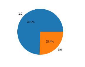
Pie chart for the distribution of the data within two class

Oh! the data imbalance. We will have to deal with this problem otherwise the model trained on this dataset will have a harder time predicting positive classes which is our main objective here.

Model Training

Now we will separate the features and target variables and split them into training and the testing data by using which we will select the model which is performing best on the validation data.

Python3

features = df.drop('class', axis=1)
target = df['class']

X_train, X_val,\
    Y_train, Y_val = train_test_split(features, target,
                                      test_size=0.2,
                                      random_state=10)
X_train.shape, X_val.shape

Output:

((201, 30), (51, 30))

Handling the data imbalance problem by using the over-sampling method on the minority class.

Python3

# As the data was highly imbalanced we will balance
#  it by adding repetitive rows of minority class.
ros = RandomOverSampler(sampling_strategy='minority',
                        random_state=0)
X, Y = ros.fit_resample(X_train, Y_train)
X.shape, Y.shape

Output:

((302, 30), (302,))

The dataset has been already normalized in the data cleaning step we can directly train some state-of-the-art machine learning models and compare them which fit better with our data.

Python3

from sklearn.metrics import roc_auc_score as ras
models = [LogisticRegression(), XGBClassifier(), SVC(kernel='rbf')]

for i in range(len(models)):
    models[i].fit(X, Y)

    print(f'{models[i]} : ')

    train_preds = models[i].predict_proba(X)[:, 1]
    print('Training Accuracy : ', ras(Y, train_preds))

    val_preds = models[i].predict_proba(X_val)[:, 1]
    print('Validation Accuracy : ', ras(Y_val, val_preds))
    print()

Output:

LogisticRegression() : 
Training Accuracy :  0.8279461427130389
Validation Accuracy :  0.8127413127413127

XGBClassifier() : 
Training Accuracy :  1.0
Validation Accuracy :  0.777992277992278

SVC(probability=True) : 
Training Accuracy :  0.7104074382702513
Validation Accuracy :  0.7606177606177607

Model Evaluation

From the above accuracies, we can say that Logistic Regression and SVC() classifier perform better on the validation data with less difference between the validation and training data. Let’s plot the confusion matrix as well for the validation data using the Logistic Regression model.

Python3

metrics.plot_confusion_matrix(models[0],
                              X_val, Y_val)
plt.show()

Output:

Confusion matrix for the validation data

Python3

print(metrics.classification_report
      (Y_val, models[0].predict(X_val)))

Output:

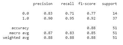
Classification report for the validation data

Conclusion:

The machine learning model we have created is around 75% to 80% accurate. The disease for which there are no diagnostics methods machine learning models are able to predict whether the person has Parkinson’s disease or not. This is the power of machine learning by using which many of the real-world problems are being solved.