OpenCV and Keras | Traffic Sign Classification for Self-Driving Car

Introduction
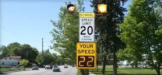
In this article, we will learn how to classify some common traffic signs that we occasionally encounter in our daily lives on the road. While building a self-driving car, it is necessary to make sure it identifies the traffic signs with a high degree of accuracy, unless the results might be catastrophic. While travelling, you may have come across numerous traffic signs, like the speed limit signal, the left or right turn signal, the stop signal and so on. Classifying all these precisely can be a daunting task, and that is where this post is going to help you.

You can get the dataset from this link – Data. It contains 4 files –

• signnames.csv – It has all the labels and their descriptors.
• train.p – It contains all the training image pixel intensities along with the labels.
• valid.p – It contains all the validation image pixel intensities along with the labels.
• test.p – It contains all the testing image pixel intensities along with the labels.

The above files with extension .p are called pickle files, which are used to serialize objects into character streams. These can be deserialized and reused later by loading them using the pickle library in python.

Let’s implement a Convolutional Neural Network (CNN) using Keras in simple and easy-to-follow steps. A CNN consists of a series of Convolutional and Pooling layers in the Neural Network which map with the input to extract features. A Convolution layer will have many filters that are mainly used to detect the low-level features such as edges of a face. The Pooling layer does dimensionality reduction to decrease computation. Moreover, it also extracts the dominant features by ignoring the side pixels. To read more about CNNs, go to this link.

Importing the libraries
We will be needing the following libraries. Make sure you install NumPy, Pandas, Keras, Matplotlib and OpenCV before implementing the following code.

import numpy as np
import matplotlib.pyplot as plt
import keras
from keras.models import Sequential
from keras.layers import Dense, Dropout, Flatten
from keras.layers.convolutional import Conv2D, MaxPooling2D
from keras.optimizers import Adam
from keras.utils.np_utils import to_categorical
from keras.preprocessing.image import ImageDataGenerator
import pickle
import pandas as pd
import random
import cv2

np.random.seed(0)

Here, we are using numpy for numerical computations, pandas for importing and managing the dataset, Keras for building the Convolutional Neural Network quickly with less code, cv2 for doing some preprocessing steps which are necessary for efficient extraction of features from the images by the CNN.

Loading the dataset
Time to load the data. We will use pandas to load signnames.csv, and pickle to load the train, validation and test pickle files. After extraction of data, it is then split using the dictionary labels “features” and “labels”.

# Read data
data = pd.read_csv("german-traffic-signs / signnames.csv")

with open('german-traffic-signs / train.p', 'rb') as f:
    train_data = pickle.load(f)
with open('german-traffic-signs / valid.p', 'rb') as f:
    val_data = pickle.load(f)
with open('german-traffic-signs / test.p', 'rb') as f:
    test_data = pickle.load(f)

# Extracting the labels from the dictionaries
X_train, y_train = train_data['features'], train_data['labels']
X_val, y_val = val_data['features'], val_data['labels']
X_test, y_test = test_data['features'], test_data['labels']

# Printing the shapes
print(X_train.shape)
print(X_val.shape)
print(X_test.shape)

Output:

(34799, 32, 32, 3)
(4410, 32, 32, 3)
(12630, 32, 32, 3)

Preprocessing the data using OpenCV
Preprocessing images before feeding into the model gives very accurate results as it helps in extracting the complex features of the image. OpenCV has some built-in functions like cvtColor() and equalizeHist() for this task. Follow the below steps for this task –

• First, the images are converted to grayscale images for reducing computation using the cvtColor() function.
• The equalizeHist() function increases the contrasts of the image by equalizing the intensities of the pixels by normalizing them with their nearby pixels.
• At the end, we normalize the pixel values between 0 and 1 by dividing them by 255.

def preprocessing(img):
    img = cv2.cvtColor(img, cv2.COLOR_BGR2GRAY)
    img = cv2.equalizeHist(img)
    img = img / 255
    return img

X_train = np.array(list(map(preprocessing, X_train)))
X_val = np.array(list(map(preprocessing, X_val)))
X_test = np.array(list(map(preprocessing, X_test)))

X_train = X_train.reshape(34799, 32, 32, 1)
X_val = X_val.reshape(4410, 32, 32, 1)
X_test = X_test.reshape(12630, 32, 32, 1)

After reshaping the arrays, it’s time to feed them into the model for training. But to increase the accuracy of our CNN model, we will involve one more step of generating augmented images using the ImageDataGenerator.

This is done to reduce overfitting the training data as getting more varied data will result in a better model. The value 0.1 is interpreted as 10%, whereas 10 is the degree of rotation. We are also converting the labels to categorical values, as we normally do.

datagen = ImageDataGenerator(width_shift_range = 0.1,
                  height_shift_range = 0.1,
                  zoom_range = 0.2,
                  shear_range = 0.1,
                  rotation_range = 10)
datagen.fit(X_train)

y_train = to_categorical(y_train, 43)
y_val = to_categorical(y_val, 43)
y_test = to_categorical(y_test, 43)

Building the model
As we have 43 classes of images in the dataset, we are setting num_classes as 43. The model contains two Conv2D layers followed by one MaxPooling2D layer. This is done two times for the effective extraction of features, which is followed by the Dense layers. A dropout layer of 0.5 is added to avoid overfitting the data.

num_classes = 43

def cnn_model():
    model = Sequential()
    model.add(Conv2D(60, (5, 5),
                     input_shape =(32, 32, 1),
                     activation ='relu'))

    model.add(Conv2D(60, (5, 5), activation ='relu'))
    model.add(MaxPooling2D(pool_size =(2, 2)))

    model.add(Conv2D(30, (3, 3), activation ='relu'))
    model.add(Conv2D(30, (3, 3), activation ='relu'))
    model.add(MaxPooling2D(pool_size =(2, 2)))

    model.add(Flatten())
    model.add(Dense(500, activation ='relu'))
    model.add(Dropout(0.5))
    model.add(Dense(num_classes, activation ='softmax'))

    # Compile model
    model.compile(Adam(lr = 0.001),
                  loss ='categorical_crossentropy',
                  metrics =['accuracy'])
    return model

model = cnn_model()
history = model.fit_generator(datagen.flow(X_train, y_train,
                            batch_size = 50), steps_per_epoch = 2000,
                            epochs = 10, validation_data =(X_val, y_val),
                            shuffle = 1)

Output:
Epoch 1/10
2000/2000 [==============================] - 129s 65ms/step - loss: 0.9130 - acc: 0.7322 - val_loss: 0.0984 - val_acc: 0.9669
Epoch 2/10
2000/2000 [==============================] - 119s 60ms/step - loss: 0.2084 - acc: 0.9352 - val_loss: 0.0609 - val_acc: 0.9803
Epoch 3/10
2000/2000 [==============================] - 116s 58ms/step - loss: 0.1399 - acc: 0.9562 - val_loss: 0.0409 - val_acc: 0.9878
Epoch 4/10
2000/2000 [==============================] - 115s 58ms/step - loss: 0.1066 - acc: 0.9672 - val_loss: 0.0262 - val_acc: 0.9925
Epoch 5/10
2000/2000 [==============================] - 116s 58ms/step - loss: 0.0890 - acc: 0.9726 - val_loss: 0.0268 - val_acc: 0.9925
Epoch 6/10
2000/2000 [==============================] - 115s 58ms/step - loss: 0.0777 - acc: 0.9756 - val_loss: 0.0237 - val_acc: 0.9927
Epoch 7/10
2000/2000 [==============================] - 132s 66ms/step - loss: 0.0700 - acc: 0.9779 - val_loss: 0.0327 - val_acc: 0.9900
Epoch 8/10
2000/2000 [==============================] - 122s 61ms/step - loss: 0.0618 - acc: 0.9812 - val_loss: 0.0267 - val_acc: 0.9914
Epoch 9/10
2000/2000 [==============================] - 115s 57ms/step - loss: 0.0565 - acc: 0.9830 - val_loss: 0.0146 - val_acc: 0.9957
Epoch 10/10
2000/2000 [==============================] - 120s 60ms/step - loss: 0.0577 - acc: 0.9828 - val_loss: 0.0222 - val_acc: 0.9939

After successfully compiling the model, and fitting in on the train and validation data, let us evaluate it by using Matplotlib.

Evaluation and testing
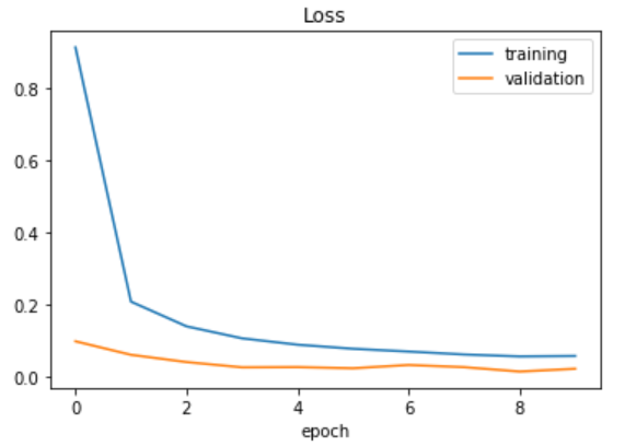
Plotting the loss function.

plt.plot(history.history['loss'])
plt.plot(history.history['val_loss'])
plt.legend(['training', 'validation'])
plt.title('Loss')
plt.xlabel('epoch')

Output:

Plotting the accuracy function.

plt.plot(history.history['acc'])
plt.plot(history.history['val_acc'])
plt.legend(['training', 'validation'])
plt.title('Accuracy')
plt.xlabel('epoch')

Output:

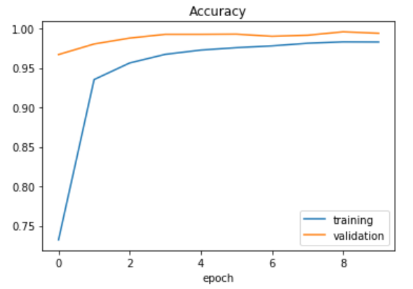
As you can see, we have fitted the data well keeping both the training and validation loss at a minimum. Time to evaluate how our model performs on the test data.

score = model.evaluate(X_test, y_test, verbose = 0)
print('Test Loss: ', score[0])
print('Test Accuracy: ', score[1])

Output:

Test Loss:  0.16352852963907774
Test Accuracy:  0.9701504354899777

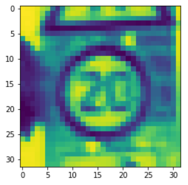
Let us check one test image by feeding it into the model. The model gives a prediction of class 0 (Speed limit 20), which is correct.

plt.imshow(X_test[990].reshape(32, 32))
print("Predicted sign: "+ str(
        model.predict_classes(X_test[990].reshape(1, 32, 32, 1))))

Output:
Predicted sign: [0]