Ola Bike Ride Request Forecast using ML

From telling rickshaw-wala where to go, to tell him where to come we have grown up. Yes, we are talking about online cab and bike facility providers like OLA and Uber. If you had used this app some times then you must have paid some day less and someday more for the same journey. But have you ever thought what is the reason behind it? It is because of the high demand at some hours. this is not the only factor but this is one of them.

Ola Bike Ride Request Forecast using ML

In this article, we will try to predict ride-request for a particular hour using machine learning. One can refer to the below explanation for the column names in the dataset and their values as well.

season

1. spring
2. summer
3. fall
4. winter

weather

1. Clear, Few clouds, Partly cloudy, Partly cloudy
2. Mist + Cloudy, Mist + Broken clouds, Mist + Few clouds, Mist
3. Light Snow, Light Rain + Thunderstorm + Scattered clouds, Light Rain + Scattered clouds
4. Heavy Rain + Ice Pallets + Thunderstorm + Mist, Snow + Fog

casual – number of non-registered user rentals initiated
registered – number of registered user rentals initiated
count – number of ride request raised on the app for that particular hour.

Importing Libraries and Dataset

Python libraries make it easy for us to handle the data and perform typical and complex tasks with a single line of code.

• Pandas – This library helps to load the data frame in a 2D array format and has multiple functions to perform analysis tasks in one go.
• Numpy – Numpy arrays are very fast and can perform large computations in a very short time.
• Matplotlib/Seaborn – This library is used to draw visualizations.
• Sklearn – This module contains multiple libraries are having pre-implemented functions to perform tasks from data preprocessing to model development and evaluation.
• XGBoost – This contains the eXtreme Gradient Boosting machine learning algorithm which is one of the algorithms which helps us to achieve high accuracy on predictions.

Python3

import numpy as np
import pandas as pd
import matplotlib.pyplot as plt
import seaborn as sb
from sklearn.model_selection import train_test_split
from sklearn.preprocessing import LabelEncoder, StandardScaler
from sklearn import metrics
from sklearn.svm import SVC
from xgboost import XGBRegressor
from sklearn.linear_model import LinearRegression, Lasso, Ridge
from sklearn.ensemble import RandomForestRegressor

import warnings
warnings.filterwarnings('ignore')

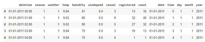
Now let’s load the dataset into the panda’s data frame and print its first five rows.

Python3

df = pd.read_csv('ola.csv')
df.head()

Output:

First five rows of the dataset.

Now let’s check the size of the dataset.

Python3

df.shape

Output:

(10886, 9)

Let’s check which column of the dataset contains which type of data.

Python3

df.info()

Output:

Information regarding data in the columns

As per the above information regarding the data in each column we can observe that there are no null values.

Python3

df.describe().T

Output:

Descriptive statistical measures of the dataset

Feature Engineering

There are times when multiple features are provided in the same feature or we have to derive some features from the existing ones. We will also try to include some extra features in our dataset so, that we can derive some interesting insights from the data we have. Also if the features derived are meaningful then they become a deciding factor in increasing the model’s accuracy significantly.

Python3

parts = df["datetime"].str.split(" ", n=2, expand=True)
df["date"] = parts[0]
df["time"] = parts[1].str[:2].astype('int')
df.head()

Output:

Addition of date and time feature

In the above step, we have separated the date and time. Now let’s extract the day, month, and year from the date column.

Python3

parts = df["date"].str.split("-", n=3, expand=True)
df["day"] = parts[0].astype('int')
df["month"] = parts[1].astype('int')
df["year"] = parts[2].astype('int')
df.head()

Output:

Addition of day, month and year feature

Whether it is a weekend or a weekday must have some effect on the ride request count.

Python3

from datetime import datetime
import calendar


def weekend_or_weekday(year, month, day):

    d = datetime(year, month, day)
    if d.weekday() > 4:
        return 0
    else:
        return 1


df['weekday'] = df.apply(lambda x:
                         weekend_or_weekday(x['year'],
                                            x['month'],
                                            x['day']),
                         axis=1)
df.head()

Output:

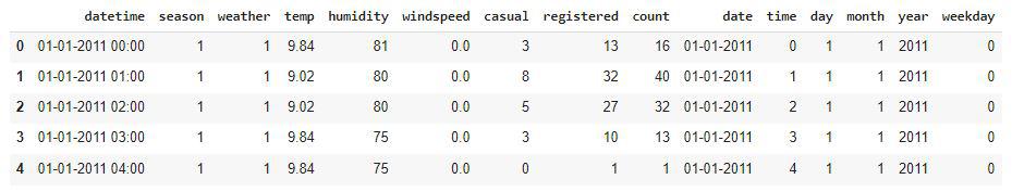
Addition of a weekday feature

Bike ride demands are also affected by whether it is am or pm.

Python3

def am_or_pm(x):
    if x > 11:
        return 1
    else:
        return 0


df['am_or_pm'] = df['time'].apply(am_or_pm)
df.head()

Output:

Addition of feature including am or pm information

It would be nice to have a column which can indicate whether there was any holiday on a particular day or not.

Python3

from datetime import date
import holidays


def is_holiday(x):

    india_holidays = holidays.country_holidays('IN')

    if india_holidays.get(x):
        return 1
    else:
        return 0


df['holidays'] = df['date'].apply(is_holiday)
df.head()

Output:

Addition of feature including holiday information

Now let’s remove the columns which are not useful for us.

Python3

df.drop(['datetime', 'date'],
        axis=1,
        inplace=True)

There may be some other relevant features as well which can be added to this dataset but let’s try to build a build with these ones and try to extract some insights as well.

Exploratory Data Analysis

EDA is an approach to analyzing the data using visual techniques. It is used to discover trends, and patterns, or to check assumptions with the help of statistical summaries and graphical representations. 

We have added some features to our dataset using some assumptions. Now let’s check what are the relations between different features with the target feature.

Python3

df.isnull().sum()

Output:

Sum of null values present in each column

Now, we will check for any relation between the ride request count with respect to the day, time, or month.

Python3

features = ['day', 'time', 'month']

plt.subplots(figsize=(15, 10))
for i, col in enumerate(features):
    plt.subplot(2, 2, i + 1)
    df.groupby(col).mean()['count'].plot()
plt.show()

Output:

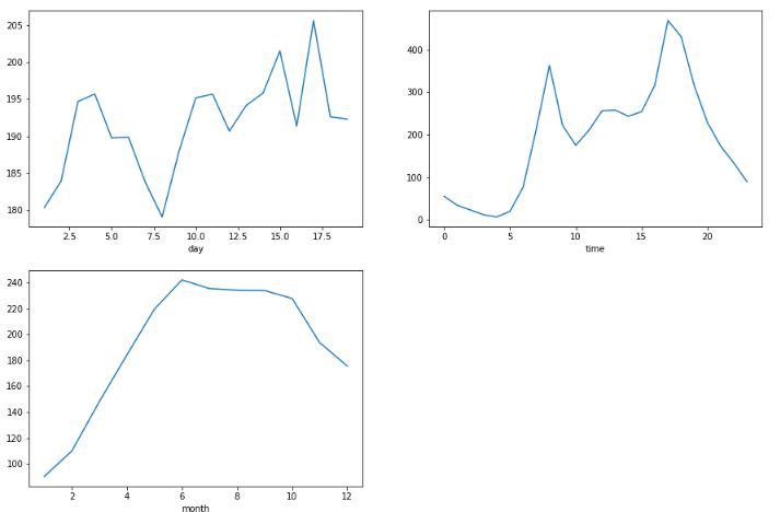
Line plot for the average count of ride requests

From the above line plots we can confirm some real-life observations:

• There is no such pattern in the day-wise average of the ride requests.
• More ride requests in the working hours as compared to the non-working hours.
• The average ride request count has dropped in the month of festivals that is after the 7th month that is July that is due to more holidays in these months.

Python3

features = ['season', 'weather', 'holidays',\
            'am_or_pm', 'year', 'weekday']

plt.subplots(figsize=(20, 10))
for i, col in enumerate(features):
    plt.subplot(2, 3, i + 1)
    df.groupby(col).mean()['count'].plot.bar()
plt.show()

Output:

Bar plot for the average count of the ride request

From the above bar plots we can confirm some real-life observations:

• Ride request demand is high in the summer as well as season.
• The third category was extreme weather conditions due to this people avoid taking bike rides and like to stay safe at home.
• On holidays no college or offices are open due to this ride request demand is low.
• More ride requests during working hours as compared to non-working hours.
• Bike ride requests have increased significantly from the year 2011 to the year 2012.

Python3

features = ['temp', 'windspeed']

plt.subplots(figsize=(15, 5))
for i, col in enumerate(features):
  plt.subplot(1, 2, i + 1)
  sb.distplot(df[col])
plt.show()

Output:

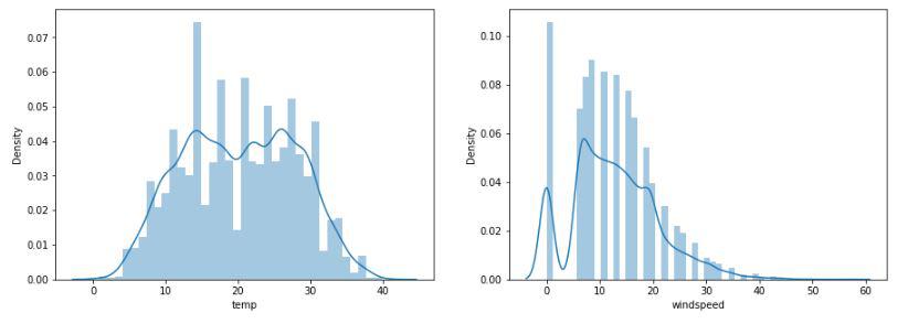
Distribution plot to visualize the data distribution for some columns

Temperature values are normally distributed but due to the high number of 0 entries in the windspeed column, the data distribution shows some irregularities.

Python

features = ['temp', 'windspeed']

plt.subplots(figsize=(15, 5))
for i, col in enumerate(features):
  plt.subplot(1, 2, i + 1)
  sb.boxplot(df[col])
plt.show()

Output:

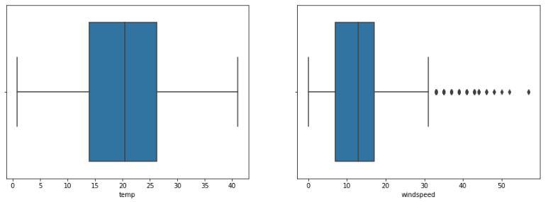
Box plot to detect the outliers present in the data

Ah! outliers let’s check how much data we will lose if we remove outliers.

Python3

num_rows = df.shape[0] - df[df['windspeed']<32].shape[0]
print(f'Number of rows that will be lost if we remove outliers is equal to {num_rows}.')

Output:

Number of rows that will be lost if we remove outliers is equal to 227.

We can remove this many rows because we have around 10000 rows of data so, this much data loss won’t affect the learning for our model.

Python3

features = ['humidity', 'casual', 'registered', 'count']

plt.subplots(figsize=(15, 10))
for i, col in enumerate(features):
    plt.subplot(2, 2, i + 1)
    sb.boxplot(df[col])
plt.show()

Output:

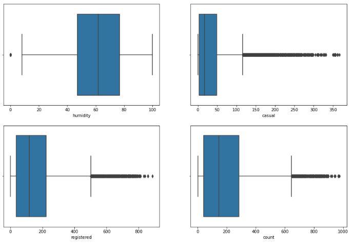
Box plot to detect the outliers present in the data

Now let’s check whether there are any highly correlated features in our dataset or not. 

Python3

sb.heatmap(df.corr() > 0.8,
           annot=True,
           cbar=False)
plt.show()

Output:

Heatmap to detect the highly correlated features

Here the registered feature is highly correlated with our target variable which is count. This will lead to a situation of data leakage if we do not handle this situation. So, let’s remove this ‘registered’ column from our feature set and also the ‘time’ feature.

Now, we have to remove the outliers we found in the above two observations that are for the humidity and wind speed.

Python3

df.drop(['registered', 'time'], axis=1, inplace=True)
df = df[(df['windspeed'] < 32) & (df['humidity'] > 0)]

Model Training

Now we will separate the features and target variables and split them into training and the testing data by using which we will select the model which is performing best on the validation data.

Python3

features = df.drop(['count'], axis=1)
target = df['count'].values

X_train, X_val, Y_train, Y_val = train_test_split(features,
                                                  target,
                                                  test_size = 0.1,
                                                  random_state=22)
X_train.shape, X_val.shape

Output:

((9574, 12), (1064, 12))

Normalizing the data before feeding it into machine learning models helps us to achieve stable and fast training.

Python3

scaler = StandardScaler()
X_train = scaler.fit_transform(X_train)
X_val = scaler.transform(X_val)

We have split our data into training and validation data also the normalization of the data has been done. Now let’s train some state-of-the-art machine learning models and select the best out of them using the validation dataset.

Python3

from sklearn.metrics import mean_absolute_error as mae
models = [LinearRegression(), XGBRegressor(), Lasso(),
          RandomForestRegressor(), Ridge()]

for i in range(5):
    models[i].fit(X_train, Y_train)

    print(f'{models[i]} : ')

    train_preds = models[i].predict(X_train)
    print('Training Error : ', mae(Y_train, train_preds))

    val_preds = models[i].predict(X_val)
    print('Validation Error : ', mae(Y_val, val_preds))
    print()

Output:

LinearRegression() : 
Training Error :  82.16822894994276
Validation Error :  81.8305740004507

XGBRegressor() : 
Training Error :  63.11707474538795
Validation Error :  63.42360674337785

Lasso() : 
Training Error :  81.88956971312291
Validation Error :  81.54215896838741

RandomForestRegressor() : 
Training Error :  22.467302366528397
Validation Error :  59.77688589778017

Ridge() : 
Training Error :  82.16648310000349
Validation Error :  81.82943228466443

The predictions made by the RandomForestRegressor are really amazing compared to the other model. In the case of RandomForestRegressor, there is a little bit of overfitting but we can manage it by hyperparameter tuning.